Edwin Jan Klein - Universiteit Twente

More documents

Recommendations

Info

Chapter 4 Listing 4.3. Pseudo code for the calculation function of waveguide primitive. (time propagating primitive) Calculate() { If a new value has been placed on port 1 { Multiply the value at port 1 with the waveguide attenuation and the phase delay (eq. 2.9) to obtain the value ‘V2’ at port 2; } } Calculate the time delay dT of the signal within the waveguide; Find the port ‘C2’ that is connected to port 2; Find the primitive ‘P2’ that is the parent of this port; Tell the scheduler to put the value V2 into port C2 after expiration time delay dT; //The scheduler will call Calculate() of primitive P2 If a new value has been placed on port 2 { …………………… } 4.5.2.2 The execution engine Although the primitives perform all the important calculations the scheduler is critical to the flow of these calculations. The scheduler performs only three simple but very important tasks: • The initialization of the dataflow. One of the main strengths of the simulation method used by Aurora is that it only reacts to changes within the optical system that is being simulated. Each primitive can only call (directly or through the scheduler) the calculation functions of the primitives that are connected to it. A change in a signal on one of the ports of a primitive (followed by calling the calculate() function of that primitive) will therefore only ever affect the signals going through all the primitives that are directly or indirectly connected to this primitive. This makes the method highly efficient at simulating large components or even large optical networks where there may be many subsections that are not connected in any way. Because the simulation is change driven this also implies that a simulation can only start after an initial signal change is made on one of the nodes in the optical system that is being simulated. At the start of a simulation the execution engine therefore gives an initial change to designated nodes to initialize the flow of data. • Callback storage and execution. When the simulation is running the execution engine accepts the calls of all timed primitives and stores these calls in order in a list as shown in Figure 4.12. In this list all the calls are sorted by time. When the simulation time has progressed to a time that is equal to the call-time of these calls the engine 88
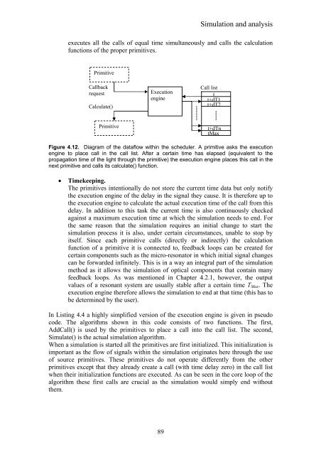
89 Simulation and analysis executes all the calls of equal time simultaneously and calls the calculation functions of the proper primitives. Primitive Callback request Calculate() Primitive Execution engine Call list t t+dT1 t+dT2 t+dTn tMax Figure 4.12. Diagram of the dataflow within the scheduler. A primitive asks the execution engine to place call in the call list. After a certain time has elapsed (equivalent to the propagation time of the light through the primitive) the execution engine places this call in the next primitive and calls its calculate() function. • Timekeeping. The primitives intentionally do not store the current time data but only notify the execution engine of the delay in the signal they cause. It is therefore up to the execution engine to calculate the actual execution time of the call from this delay. In addition to this task the current time is also continuously checked against a maximum execution time at which the simulation needs to end. For the same reason that the simulation requires an initial change to start the simulation process it is also, under certain circumstances, unable to stop by itself. Since each primitive calls (directly or indirectly) the calculation function of a primitive it is connected to, feedback loops can be created for certain components such as the micro-resonator in which initial signal changes can be forwarded infinitely. This is in a way an integral part of the simulation method as it allows the simulation of optical components that contain many feedback loops. As was mentioned in Chapter 4.2.1, however, the output values of a resonant system are usually stable after a certain time TMax. The execution engine therefore allows the simulation to end at that time (this has to be determined by the user). In Listing 4.4 a highly simplified version of the execution engine is given in pseudo code. The algorithms shown in this code consists of two functions. The first, AddCall() is used by the primitives to place a call into the call list. The second, Simulate() is the actual simulation algorithm. When a simulation is started all the primitives are first initialized. This initialization is important as the flow of signals within the simulation originates here through the use of source primitives. These primitives do not operate differently from the other primitives except that they already create a call (with time delay zero) in the call list when their initialization functions are executed. As can be seen in the core loop of the algorithm these first calls are crucial as the simulation would simply end without them.
Page 1 and 2:
DENSELY INTEGRATED MICRORING- RESON
Page 3 and 4:
DENSELY INTEGRATED MICRORING- RESON
Page 5:
To my parents…
Page 8 and 9:
esonators is limited by the spacing
Page 10 and 11:
iv Samenvatting Dit proefschrift be
Page 12 and 13:
schakelaar “aan” is, dan is de
Page 14 and 15:
3.6.2 Overlap loss reduction.......
Page 17 and 18:
Chapter 1 Introduction The devices
Page 19 and 20:
1.2 Broadband to the home 3 Introdu
Page 21 and 22:
1.3 Bringing Fiber to the Home 5 In
Page 23 and 24:
Figure 1.5. The technological scope
Page 25:
9 Introduction these basic paramete
Page 28 and 29:
Chapter 2 2.1 Introduction Integrat
Page 30 and 31:
Chapter 2 light Icav2 in the cavity
Page 32 and 33:
Chapter 2 ∆ = ⎛ β r − β g
Page 34 and 35:
Chapter 2 2.3.3 Combined model The
Page 36 and 37:
Chapter 2 FC 4µ 1µ 2 ⋅ χr = 2
Page 38 and 39:
Chapter 2 P Through /P In (dB) 0 -1
Page 40 and 41:
Chapter 2 The figure shows that it
Page 42 and 43:
Chapter 2 In − jϕr1 2 Figure 2.1
Page 44 and 45:
Chapter 2 differences between the f
Page 46 and 47:
Chapter 2 M = ⋅ FSR = N ⋅ FSR F
Page 48 and 49:
Chapter 2 the heat will therefore f
Page 50 and 51:
Chapter 2 index. Although this can
Page 52 and 53:
Chapter 2 resonators for instance h
Page 54 and 55: Chapter 2 a rather complex MEMS bas
Page 56 and 57: Chapter 3 3.1 Introduction The most
Page 58 and 59: Chapter 3 3.2.1 Drop port on-resona
Page 60 and 61: Chapter 3 3.2.3 Filter bandwidth In
Page 62 and 63: Chapter 3 (resulting in a higher ba
Page 64 and 65: Chapter 3 Figure 3.11. Residual cha
Page 66 and 67: Chapter 3 3.3 Geometrical design ch
Page 68 and 69: Chapter 3 resonator and the port wa
Page 70 and 71: Chapter 3 Another important fact wh
Page 72 and 73: Chapter 3 The flowchart of the desi
Page 74 and 75: Chapter 3 While the resonator in th
Page 76 and 77: Chapter 3 3.6.1 Port waveguide and
Page 78 and 79: Chapter 3 overlap losses are only 0
Page 80 and 81: Chapter 3 3.7 Component design cons
Page 82 and 83: Chapter 3 By maximizing the power t
Page 84 and 85: Chapter 3 important, due to the fac
Page 86 and 87: Chapter 4 4.1 Introduction As was s
Page 88 and 89: Chapter 4 4.2.1 Transient response
Page 90 and 91: Chapter 4 Under the condition that
Page 92 and 93: Chapter 4 Figure 4.4. Screenshot of
Page 94 and 95: Chapter 4 The equations required to
Page 96 and 97: Chapter 4 using an approach based o
Page 98 and 99: Chapter 4 4.5.1 Architecture The Au
Page 100 and 101: Chapter 4 4.5.2 Simulation method A
Page 102 and 103: Chapter 4 Figure 4.9. A Primitive w
Page 106 and 107: Chapter 4 Listing 4.4. Pseudo code
Page 108 and 109: Chapter 4 simulated output spectra
Page 110 and 111: Chapter 4 Figure 4.21. The reflecto
Page 112 and 113: Chapter 4 P Drop /P In (dB) 0 -10 -
Page 114 and 115: Chapter 4 Figure 4.27a. OADM with r
Page 116 and 117: Chapter 4 will propagate through th
Page 118 and 119: Chapter 4 As demonstrated by these
Page 120 and 121: Chapter 4 What is more interesting
Page 122 and 123: Chapter 4 method it does allow time
Page 124 and 125: Chapter 4 complex than the interact
Page 126 and 127: Chapter 5 5.1 Introduction The mate
Page 128 and 129: Chapter 5 wafer is used (step 1). T
Page 130 and 131: Chapter 5 range of 0.9 to 1.1 µm.
Page 132 and 133: Chapter 5 The process flow with the
Page 134 and 135: Chapter 5 5.3.3 Mask layout The big
Page 136 and 137: Chapter 5 5.4. Fabrication and mask
Page 138 and 139: Chapter 5 1. Definition of the vert
Page 140 and 141: Chapter 5 5.4.2 Fabrication The fab
Page 142 and 143: Chapter 5 Figure 5.21. Process flow
Page 144 and 145: Chapter 5 removed using lift-off of
Page 146 and 147: Chapter 6 6.1 Introduction About ha
Page 148 and 149: Chapter 6 In early, comparatively s
Page 150 and 151: Chapter 6 that the TEOS has a very
Page 152 and 153: Chapter 6 The most important aspect
Page 154 and 155:
Chapter 6 6.2.3 Chromium heater des
Page 156 and 157:
Chapter 6 Therefore, even if the si
Page 158 and 159:
Chapter 6 Next, the heater was heat
Page 160 and 161:
Chapter 6 6.3 Characterization of s
Page 162 and 163:
Chapter 6 polarization maintaining
Page 164 and 165:
Chapter 6 the resonators in this gr
Page 166 and 167:
Chapter 6 Although the fitted coupl
Page 168 and 169:
Chapter 6 a cladding thickness of 3
Page 170 and 171:
Chapter 6 6.4 A wavelength selectiv
Page 172 and 173:
Chapter 6 A possible explanation fo
Page 175 and 176:
Chapter 7 Densely integrated device
Page 177 and 178:
Densely integrated devices for WDM-
Page 179 and 180:
Page 181 and 182:
Page 183 and 184:
7.2.2 Spectral measurements Densely
Page 185 and 186:
Page 187 and 188:
Page 189 and 190:
Power Densely integrated devices fo
Page 191 and 192:
7.3.4 Characterization Densely inte
Page 193 and 194:
Page 195 and 196:
Figure 7.31a. Eye pattern of the re
Page 197:
Page 200 and 201:
Chapter 8 8.1 Introduction In most
Page 202 and 203:
Chapter 8 amount of power will be d
Page 204 and 205:
Chapter 8 Another problem that may
Page 206 and 207:
Chapter 8 halves that are each comp
Page 209 and 210:
Chapter 9 Discussion and Conclusion
Page 211 and 212:
Appendix A. Mason’s rule Several
Page 213 and 214:
Appendix B. Crosstalk Derivation Th
Page 215 and 216:
List of Acronyms ADSL - Asymmetric
Page 217 and 218:
List of Symbols Q - Quality Factor
Page 219 and 220:
Bibliography [1] Dan Schiller, “E
Page 221 and 222:
Regions,” IEEE Photonics Technolo
Page 223 and 224:
[66] B. E. Little, S. T. Chu, J. V.
Page 225 and 226:
[97] H. Haeiwa, T. Naganawa and Y.
Page 227 and 228:
[135] A. Driessen, D. H. Geuzebroek
Page 229 and 230:
[165] T. Barwicz, M. R. Watts, M. A
Page 231 and 232:
Publication List Patents (pending)
Page 233 and 234:
R. Dekker, L.T.H.Hilderink, M.B.J.
Page 235 and 236:
Networks (BB Photonics),” Interna
Page 237 and 238:
Dankwoord/Acknowledgements Zo, dit
Page 239:
223
show all

Edwin Jan Klein - Universiteit Twente

You also want an ePaper? Increase the reach of your titles

Delete template?

Save as template?