Edwin Jan Klein - Universiteit Twente

In
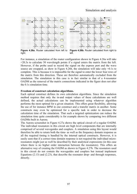
Figure 4.26a. Router calculated from left to
right.
97
Matrix
connections
Simulation and analysis
Figure 4.26b. Router calculated from right to
left.
For instance, a simulation of the router configuration shown in Figure 4.26a will take
≈20.3s to calculate 50 wavelength points if a signal enters the matrix from the left.
However, if the probe used to record the signal on the express port and the wave
source are swapped, as show in Figure 4.26b, the simulation will take only ≈0.1s to
complete. This is because it is impossible for the signal to enter the lower four rows of
the matrix from this direction. These are therefore automatically excluded from the
simulation. The simulation in this case is in fact similar to that of a 4-resonator
OADM as the removal of the matrix connections indicated in the figure does not alter
the 0.1s simulation time.
Freedom of construct calculation algorithms.
Each optical construct defines its own calculation algorithms. Since the simulation
method requires that only the in-and output values of these calculations are well
defined, the actual calculations can be implemented using whatever algorithm
performs the most optimal for a given situation. This offers great flexibility, allowing
the use of for instance BPM in one construct and a transfer matrix in another. Some
constructs may even be optimized for a specific task in order to decrease the
calculation time of the simulation. That such a targeted optimization can reduce the
simulation time quite considerably is for example shown by comparing two different
OADMs built in Aurora.
The Aurora screenshot in Figure 4.27a shows the optical circuit of a regular OADM.
The individual resonators in this circuit are high level components that are internally
comprised of several waveguides and couplers. A simulation using this layout would
therefore be able to return both the time- as well as the frequency domain response as
all the required timing is handled by the internal optical constructs. However, it is
easily seen that if a correct time domain response is not required the individual microresonators
might just as well be described by their analytical expressions (in this case
where there is no higher order interaction between the resonators). This offers an
alternative way of creating the OADM as shown in Figure 4.27b. The resonators used
in this circuit do not contain the waveguides and couplers but instead implement
Equations (2.13) and (2.23), that describe the resonator drop- and through responses,
directly.
In