Edwin Jan Klein - Universiteit Twente

Chapter 4
Listing 4.4. Pseudo code implementation of the execution engine.
AddCall(dT, V, C)
{
Create the call with value V and port target C to the call list at time TCurr+dT;
}
Simulate()
{
Set the current time TCurr to 0;
Initialize all the primitives;
Find the first call in the call list;
TCurr is now equal to the time in this call;
}
loop //Simulation loop
{
Execute all the calls that have time TCurr by
First placing the forwarded signal values V in these calls on their
target nodes C;
Then calling the Calculate() functions of the parent primitives of these nodes;
Find the first call that has a time> TCurr in the call list;
TCurr is now equal to the time in this call;
} until TCurr>TMax or until there are no more calls;
With these first calls, however, the core loop of the algorithm becomes self
sustaining: If the algorithm executes the calculate functions of the primitives that
these first calls refer to, these in turn will either generate one or more new calls
themselves or, if they are instantaneous, call another primitives that do so. When the
core loop has finished executing all the calls placed at TCurr=0 it can then simply
continue with the newly created calls that are next on the time line. These calls in turn
will then generate their own new calls and so forth and so on.
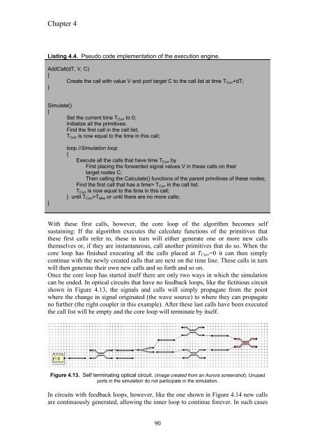
Once the core loop has started itself there are only two ways in which the simulation
can be ended. In optical circuits that have no feedback loops, like the fictitious circuit
shown in Figure 4.13, the signals and calls will simply propagate from the point
where the change in signal originated (the wave source) to where they can propagate
no further (the right coupler in this example). After these last calls have been executed
the call list will be empty and the core loop will terminate by itself.
Figure 4.13. Self terminating optical circuit. (Image created from an Aurora screenshot). Unused
ports in the simulation do not participate in the simulation.
In circuits with feedback loops, however, like the one shown in Figure 4.14 new calls
are continuously generated, allowing the inner loop to continue forever. In such cases
90