Edwin Jan Klein - Universiteit Twente

Chapter 4
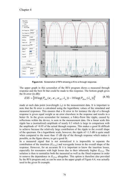
Figure 4.4. Screenshot of RFit showing a fit to a through response.
The upper graph in this screenshot of the RFit program shows a measured through
response and the best fit that could be made to this response. The bottom graph gives
the fit error (in dB):
(4.16)
[ ] 2
log( P ( κ , κ , α , λ )) − 10 log( P ( ))
ESS = 10 Sim
dB m
Meas λm
1
2
made at each data point (wavelength λm) in the measurement data. It is important to
note that the fit error is calculated using the logarithmic values of the simulated and
measured responses. This ensures that a fit error in for instance the dip of a through
response is given equal weight as an error elsewhere in the response and results in a
better fit. In the given screenshot for instance, a Fabry-Perot like ripple, caused by
reflections within the device, is seen in the measurement data. On a linear scale this
ripple has a (normalized) amplitude of nearly 0.3 which is large in comparison with
the amplitude of ≈0.95 of the actual through response. This makes a good fit difficult
to achieve because the relatively large contribution of the ripple to the overall shape
of the spectrum. On a logarithmic scale, however, the ripple of ≈1.5 dB is quite small
when compared to the more than 15 dB dip of the through response which makes it
possible, as the figure shows, to get a good fit.
In a measured signal that is not normalized it is impossible to separate the
contribution of the insertion (ILDrop) and waveguide losses in the overall shape of the
response. However, for an accurate fit it is important to know the insertion losses,
especially for resonators with high losses due to their inherently higher ILDrop. The
solution is then to normalize both the measured as well as the fitted response in order
to remove the dependence in ILDrop altogether. This option is therefore also provided
by the RFit program and, as can be seen in the upper graph of Figure 4.4, was actually
used in the given fit example.
76