Edwin Jan Klein - Universiteit Twente

47
Design
In most cases, rather than a single channel there will be multiple channels on the bus
so that the resonators cannot be tuned to be maximally off for all channels. In these
cases the power that is extracted from a channel on the bus can be calculated using:
IL
2
2 2
⎛ µ
⎞
1 − 2χ
r ⋅ µ 1µ
2 ⋅ cos( 2π
⋅ ∆λcr
/ FSR)
+ χ r ⋅ µ 2
= −10log
⎜
⎟
2 2
⎝1
− 2χ
r ⋅ µ 1µ
2 ⋅ cos( 2π
⋅ ∆λcr
/ FSR)
+ µ 1 µ 2 ⋅ χ r ⎠
Through _ ∆λ 2
(3.7)
where ∆λcr is the difference between the center wavelength of a channel on the bus
and the resonance wavelength of the resonator. In a practical application a single free
channel (i.e. a channel that is not present on the bus) might be chosen to “park” all
resonators that should not drop a signal. If the spacing between the channels is
defined as ∆λcs then ∆λcr=∆λcs.
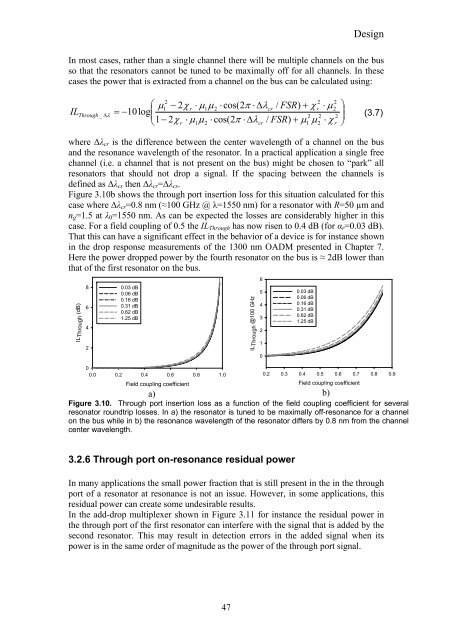
Figure 3.10b shows the through port insertion loss for this situation calculated for this
case where ∆λcr=0.8 nm (≈100 GHz @ λ=1550 nm) for a resonator with R=50 µm and
ng=1.5 at λ0=1550 nm. As can be expected the losses are considerably higher in this
case. For a field coupling of 0.5 the ILThrough has now risen to 0.4 dB (for αr=0.03 dB).
That this can have a significant effect in the behavior of a device is for instance shown
in the drop response measurements of the 1300 nm OADM presented in Chapter 7.
Here the power dropped power by the fourth resonator on the bus is ≈ 2dB lower than
that of the first resonator on the bus.
ILThrough (dB)
8 0.03 dB
0.06 dB
0.16 dB
6
0.31 dB
0.62 dB
1.25 dB
4
2
0
0.0 0.2 0.4 0.6 0.8 1.0
Field coupling coefficient
a)
b)
Figure 3.10. Through port insertion loss as a function of the field coupling coefficient for several
resonator roundtrip losses. In a) the resonator is tuned to be maximally off-resonance for a channel
on the bus while in b) the resonance wavelength of the resonator differs by 0.8 nm from the channel
center wavelength.
3.2.6 Through port on-resonance residual power
0.2 0.3 0.4 0.5 0.6 0.7 0.8 0.9
Field coupling coefficient
In many applications the small power fraction that is still present in the in the through
port of a resonator at resonance is not an issue. However, in some applications, this
residual power can create some undesirable results.
In the add-drop multiplexer shown in Figure 3.11 for instance the residual power in
the through port of the first resonator can interfere with the signal that is added by the
second resonator. This may result in detection errors in the added signal when its
power is in the same order of magnitude as the power of the through port signal.
ILThrough @100 GHz
6
5
4
3
2
1
0
0.03 dB
0.06 dB
0.16 dB
0.31 dB
0.62 dB
1.25 dB