Edwin Jan Klein - Universiteit Twente

27
The Micro-Resonator
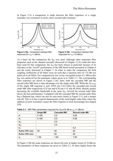
In Figure 2.16 a comparison is made between the filter responses of a single
resonator, two resonators in series, and a second order resonator.
P Drop /P In (dB)
0
-10
-20
-30
Single MR
Double MR
2nd Order MR
1548 1549 1550
Wavelength (nm)
1551 1552
Figure 2.16a. Comparison between filter
responses for αdB =1 dB/cm.
P Drop /P In (dB)
0
-10
-20
-30
-40
-50
1548 1549 1550 1551 1552
Wavelength (nm)
Single MR
Double MR
2nd Order MR
Figure 2.16b. Comparison between filter
responses for αdB =10 dB/cm.
As a basis for the comparison the SRR was used. Although other important filter
properties such as the channel crosstalk (discussed in Chapter 3.2.4) could also have
been used for this comparison, the SRR has been chosen in particular because of its
relevance to the “on/off” performance of the MR based switch presented in Chapter 6
and the router discussed in Chapter 7. In order to make the comparison the field
coupling coefficients of all filters were set such that a rejection ratio of ≈33 dB was
achieved in all filters. For comparatively low cavity waveguide losses of 1 dB/cm this
SRR was achieved for the parameter values given in to Table 2.1. The corresponding
filter responses are shown in Figure 2.16a. Here, both the cascaded MR and the
second order MR show a clear advantage over the single order MR. While the ∆λFWHM
of the single MR response is only 0.054 nm (≈6.8 GHz) the cascaded and second
order MR offer respectively 0.25 nm and 0.38 nm (≈31 and 48 GHz), thereby greatly
increasing the available bandwidth at the same SRR. Overall the second order filter
shows the best performance. Compared with the cascaded MR the second order filter
has a flattened top, which can also be seen more clearly in Figure 2.15, and a steeper
roll-off. This is in fact a typical characteristic of the serial higher order filter where the
addition of more resonators causes the filter response to look increasingly box-shaped
[54].
Table 2.1. MR Filter parameters required for SRR≈33 dB at αdB =1 dB/cm.
Single MR Cascaded MR Second order MR
κ1 0.195 0.5 0.58
κ2 0.195 0.5 0.58
κ21 0.5
κ22 0.5
κ3 0.2
Radius MR1 (µm) 50 50 50
Radius MR2 (µm) 50 50
ng 1.84 1.84 1.84
In Figure 2.16b the same responses are shown but now at higher losses of 10 dB/cm.
The parameters of these responses are given in Table 2.2. At these higher losses the