"Life Cycle" Hypothesis of Saving: Aggregate ... - Arabictrader.com
"Life Cycle" Hypothesis of Saving: Aggregate ... - Arabictrader.com
"Life Cycle" Hypothesis of Saving: Aggregate ... - Arabictrader.com
Create successful ePaper yourself
Turn your PDF publications into a flip-book with our unique Google optimized e-Paper software.
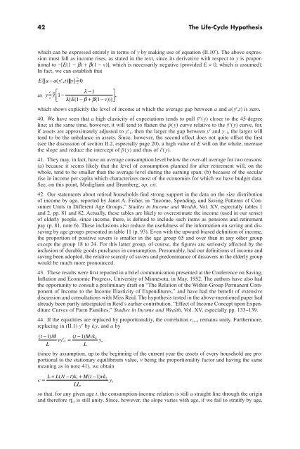
42 The <strong>Life</strong>-Cycle <strong>Hypothesis</strong><br />
which can be expressed entirely in terms <strong>of</strong> y by making use <strong>of</strong> equation (II.10¢). The above expression<br />
must fall as in<strong>com</strong>e rises, as stated in the text, since its derivative with respect to y is proportional<br />
to -[E(1 - b) + b(1 - v)], which is necessarily negative (provided E > 0, which is assumed).<br />
In fact, we can establish that<br />
e ><br />
E{ [ a- a( y , t)<br />
] y}= <<br />
0<br />
<<br />
as y= y<br />
È l -1<br />
1-<br />
˘<br />
,<br />
><br />
ÎÍ l[ E( 1- b+ b( 1-v)<br />
)]<br />
˚˙<br />
which shows explicitly the level <strong>of</strong> in<strong>com</strong>e at which the average gap between a and a(y e ,t) is zero.<br />
40. We have seen that a high elasticity <strong>of</strong> expectations tends to pull ȳ e (y) closer to the 45-degree<br />
line; at the same time, however, it will tend to flatten the p¯ (y) curve relative to the ȳ e (y) curve, for,<br />
if assets are approximately adjusted to y e -1, then the larger the gap between y e and y -1 , the larger will<br />
tend to be the unbalance in assets. Since, however, the second effect does not quite <strong>of</strong>fset the first<br />
(see the discussion <strong>of</strong> section II.2, especially page 20), a high value <strong>of</strong> E will on the whole, increase<br />
the slope and reduce the intercept <strong>of</strong> p¯ (y) and thus <strong>of</strong> c¯(y).<br />
41. They may, in fact, have an average consumption level below the over-all average for two reasons:<br />
(a) because it seems likely that the level <strong>of</strong> consumption planned for after retirement will, on the<br />
whole, tend to be smaller than the average level during the earning span; (b) because <strong>of</strong> the secular<br />
rise in in<strong>com</strong>e per capita which characterizes most <strong>of</strong> the economies for which we have budget data.<br />
See, on this point, Modigliani and Brumberg, op. cit.<br />
42. Our statements about retired households find strong support in the data on the size distribution<br />
<strong>of</strong> in<strong>com</strong>e by age, reported by Janet A. Fisher, in “In<strong>com</strong>e, Spending, and <strong>Saving</strong> Patterns <strong>of</strong> Consumer<br />
Units in Different Age Groups,” Studies in In<strong>com</strong>e and Wealth, Vol. XV, especially tables 1<br />
and 2, pp. 81 and 82. Actually, these tables are likely to overestimate the in<strong>com</strong>e (used in our sense)<br />
<strong>of</strong> elderly people, since in<strong>com</strong>e, there, is defined to include such items as pensions and retirement<br />
pay (p. 81, note 6). These inclusions also reduce the usefulness <strong>of</strong> the information on saving and dissaving<br />
by age groups presented in table 11 (p. 93). Even with the upward-biased definition <strong>of</strong> in<strong>com</strong>e,<br />
the proportion <strong>of</strong> positive savers is smaller in the age group 65 and over than in any other group<br />
except the group 18 to 24. For this latter group, <strong>of</strong> course, the figures are seriously affected by the<br />
inclusion <strong>of</strong> durable goods purchases in consumption. Presumably, had our definitions <strong>of</strong> in<strong>com</strong>e and<br />
saving been adopted, the relative scarcity <strong>of</strong> savers and predominance <strong>of</strong> dissavers in the elderly group<br />
would be much more pronounced.<br />
43. These results were first reported in a brief <strong>com</strong>munication presented at the Conference on <strong>Saving</strong>,<br />
Inflation and Economic Progress, University <strong>of</strong> Minnesota, in May, 1952. The authors have also had<br />
the opportunity to consult a preliminary draft on “The Relation <strong>of</strong> the Within-Group Permanent Component<br />
<strong>of</strong> In<strong>com</strong>e to the In<strong>com</strong>e Elasticity <strong>of</strong> Expenditures,” and have had the benefit <strong>of</strong> extensive<br />
discussion and consultations with Miss Reid. The hypothesis tested in the above-mentioned paper had<br />
already been partly anticipated in Reid’s earlier contribution, “Effect <strong>of</strong> In<strong>com</strong>e Concept upon Expenditure<br />
Curves <strong>of</strong> Farm Families,” Studies in In<strong>com</strong>e and Wealth, Vol. XV, especially pp. 133–139.<br />
44. If the equalities are replaced by proportionality, the correlation r yy-1 remains unity. Furthermore,<br />
replacing in (II.1) y e by k i y, and a by<br />
( t-1)<br />
M e<br />
( t -1)<br />
Mvk2<br />
vy-1<br />
=<br />
y,<br />
L<br />
L<br />
(since by assumption, up to the beginning <strong>of</strong> the current year the assets <strong>of</strong> every household are proportional<br />
to the stationary equilibrium value, n being the proportionality factor and having the same<br />
meaning as in note 41), we obtain<br />
L+ L( N-t) k1+ M( t-1)<br />
vk2<br />
c =<br />
y,<br />
LL<br />
t<br />
so that, for any given age t, the consumption-in<strong>com</strong>e relation is still a straight line through the origin<br />
and therefore h cy is still unity. Since, however, the slope varies with age, if we fail to stratify by age,


