- Page 1 and 2:
THE COLLECTED PAPERS OF FRANCO MODI
- Page 3 and 4:
Franco Modigliani in 1992.
- Page 5 and 6:
© 2005 Massachusetts Institute of
- Page 8 and 9:
CONTENTS Preface Francesco Franco I
- Page 10:
PREFACE The essays collected in thi
- Page 13 and 14:
xii Introduction decades of the twe
- Page 16: THE LIFE-CYCLE HYPOTHESIS I
- Page 19 and 20: 4 The Life-Cycle Hypothesis them. W
- Page 21 and 22: 6 The Life-Cycle Hypothesis which c
- Page 23 and 24: 8 The Life-Cycle Hypothesis extent
- Page 25 and 26: 10 The Life-Cycle Hypothesis Assump
- Page 27 and 28: 12 The Life-Cycle Hypothesis e dy d
- Page 29 and 30: 14 The Life-Cycle Hypothesis We wil
- Page 31 and 32: 16 The Life-Cycle Hypothesis The fi
- Page 33 and 34: 18 The Life-Cycle Hypothesis We fee
- Page 35 and 36: 20 The Life-Cycle Hypothesis P = y
- Page 37 and 38: 22 The Life-Cycle Hypothesis y y e
- Page 39 and 40: 24 The Life-Cycle Hypothesis consum
- Page 41 and 42: 26 The Life-Cycle Hypothesis as an
- Page 43 and 44: 28 The Life-Cycle Hypothesis It wil
- Page 45 and 46: 30 The Life-Cycle Hypothesis is one
- Page 47 and 48: 32 The Life-Cycle Hypothesis The re
- Page 49 and 50: 34 The Life-Cycle Hypothesis Unfort
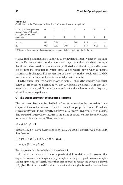
- Page 51 and 52: 36 The Life-Cycle Hypothesis basis
- Page 53 and 54: 38 The Life-Cycle Hypothesis 14. Fo
- Page 55 and 56: 40 The Life-Cycle Hypothesis 33. It
- Page 57 and 58: 42 The Life-Cycle Hypothesis which
- Page 59 and 60: 44 The Life-Cycle Hypothesis assump
- Page 62 and 63: 2 THE “LIFE-CYCLE” HYPOTHESIS O
- Page 64 and 65: The “Life-Cycle” Hypothesis of
- Page 68 and 69: The “Life-Cycle” Hypothesis of
- Page 70 and 71: The “Life-Cycle” Hypothesis of
- Page 72 and 73: (11) I C 0.634 0.080 0.634 0.092 0.
- Page 74 and 75: The “Life-Cycle” Hypothesis of
- Page 76 and 77: The “Life-Cycle” Hypothesis of
- Page 78 and 79: The “Life-Cycle” Hypothesis of
- Page 80 and 81: The “Life-Cycle” Hypothesis of
- Page 82 and 83: The “Life-Cycle” Hypothesis of
- Page 84 and 85: The “Life-Cycle” Hypothesis of
- Page 86 and 87: The “Life-Cycle” Hypothesis of
- Page 88 and 89: The “Life-Cycle” Hypothesis of
- Page 90 and 91: The “Life-Cycle” Hypothesis of
- Page 92 and 93: The “Life-Cycle” Hypothesis of
- Page 94 and 95: 3 LONG-RUN IMPLICATIONS OF ALTERNAT
- Page 96 and 97: Long-Run Implications of Alternativ
- Page 98 and 99: Long-Run Implications of Alternativ
- Page 100 and 101: Long-Run Implications of Alternativ
- Page 102 and 103: Table 3.1 A. Effects of Government
- Page 104 and 105: Long-Run Implications of Alternativ
- Page 106 and 107: Long-Run Implications of Alternativ
- Page 108 and 109: Long-Run Implications of Alternativ
- Page 110 and 111: Long-Run Implications of Alternativ
- Page 112 and 113: Long-Run Implications of Alternativ
- Page 114 and 115: Long-Run Implications of Alternativ
- Page 116 and 117:
Long-Run Implications of Alternativ
- Page 118 and 119:
Long-Run Implications of Alternativ
- Page 120 and 121:
Long-Run Implications of Alternativ
- Page 122 and 123:
4 RECENT DECLINES IN THE SAVINGS RA
- Page 124 and 125:
Table 4.1 (continued) Regression Va
- Page 126 and 127:
Recent Declines in the Savings Rate
- Page 128 and 129:
Table 4.2 (continued) First Differe
- Page 130 and 131:
Recent Declines in the Savings Rate
- Page 132 and 133:
Recent Declines in the Savings Rate
- Page 134 and 135:
Recent Declines in the Savings Rate
- Page 136 and 137:
Recent Declines in the Savings Rate
- Page 138 and 139:
Table 4.3 Period & estimation Surpl
- Page 140 and 141:
Recent Declines in the Savings Rate
- Page 142 and 143:
Recent Declines in the Savings Rate
- Page 144 and 145:
Table 4.4 The Role of Major Variabl
- Page 146 and 147:
Recent Declines in the Savings Rate
- Page 148 and 149:
Table 4.5 Estimates for Developing
- Page 150 and 151:
Table 4.6 (continued) Savings Growt
- Page 152 and 153:
Recent Declines in the Savings Rate
- Page 154 and 155:
Recent Declines in the Savings Rate
- Page 156 and 157:
5 THE AGE-SAVING PROFILE AND THE LI
- Page 158 and 159:
The Age Saving Profile 143 It is ob
- Page 160 and 161:
The Age Saving Profile 145 The exer
- Page 162 and 163:
The Age Saving Profile 147 same coh
- Page 164 and 165:
The Age Saving Profile 149 therefor
- Page 166 and 167:
The Age Saving Profile 151 One poss
- Page 168 and 169:
The Age Saving Profile 153 0 50 100
- Page 170 and 171:
The Age Saving Profile 155 0 5 10 1
- Page 172 and 173:
The Age Saving Profile 157 -10 -5 0
- Page 174 and 175:
10 40 45 Median discretionary savin
- Page 176 and 177:
The Age Saving Profile 161 effect f
- Page 178 and 179:
The Age Saving Profile 163 between
- Page 180 and 181:
The Age Saving Profile 165 tion. Si
- Page 182 and 183:
The Age Saving Profile 167 to save
- Page 184 and 185:
The Age Saving Profile 169 sampling
- Page 186 and 187:
The Age Saving Profile 171 10. One
- Page 188 and 189:
6 THE CHINESE SAVING PUZZLE AND THE
- Page 190 and 191:
Table 6.1 Chinese Household Income
- Page 192 and 193:
The Chinese Saving Puzzle 177 the p
- Page 194 and 195:
The Chinese Saving Puzzle 179 Even
- Page 196 and 197:
The Chinese Saving Puzzle 181 those
- Page 198 and 199:
The Chinese Saving Puzzle 183 3.3.2
- Page 200 and 201:
The Chinese Saving Puzzle 185 3. S(
- Page 202 and 203:
The Chinese Saving Puzzle 187 ddpCY
- Page 204 and 205:
Table 6.3 Estimates of Coefficients
- Page 206 and 207:
The Chinese Saving Puzzle 191 respe
- Page 208 and 209:
The Chinese Saving Puzzle 193 These
- Page 210 and 211:
The Chinese Saving Puzzle 195 marke
- Page 212 and 213:
The Chinese Saving Puzzle 197 coeff
- Page 214 and 215:
The Chinese Saving Puzzle 199 6 Con
- Page 216 and 217:
The Chinese Saving Puzzle 201 Accor
- Page 218 and 219:
The Chinese Saving Puzzle 203 Appen
- Page 220:
The Chinese Saving Puzzle 205 Horio
- Page 224 and 225:
7 AN ECONOMISTS’ MANIFESTO ON UNE
- Page 226 and 227:
An Economists’ Manifesto on Unemp
- Page 228 and 229:
An Economists’ Manifesto on Unemp
- Page 230 and 231:
An Economists’ Manifesto on Unemp
- Page 232 and 233:
An Economists’ Manifesto on Unemp
- Page 234 and 235:
An Economists’ Manifesto on Unemp
- Page 236 and 237:
An Economists’ Manifesto on Unemp
- Page 238 and 239:
An Economists’ Manifesto on Unemp
- Page 240 and 241:
An Economists’ Manifesto on Unemp
- Page 242 and 243:
An Economists’ Manifesto on Unemp
- Page 244 and 245:
An Economists’ Manifesto on Unemp
- Page 246 and 247:
An Economists’ Manifesto on Unemp
- Page 248 and 249:
An Economists’ Manifesto on Unemp
- Page 250 and 251:
An Economists’ Manifesto on Unemp
- Page 252:
An Economists’ Manifesto on Unemp
- Page 255 and 256:
240 Unemployment and Monetary Polic
- Page 257 and 258:
242 Unemployment and Monetary Polic
- Page 259 and 260:
244 Unemployment and Monetary Polic
- Page 261 and 262:
246 Unemployment and Monetary Polic
- Page 263 and 264:
248 Unemployment and Monetary Polic
- Page 265 and 266:
250 Unemployment and Monetary Polic
- Page 267 and 268:
252 Unemployment and Monetary Polic
- Page 269 and 270:
254 Unemployment and Monetary Polic
- Page 271 and 272:
256 Unemployment and Monetary Polic
- Page 273 and 274:
258 Unemployment and Monetary Polic
- Page 275 and 276:
260 Unemployment and Monetary Polic
- Page 277 and 278:
262 Unemployment and Monetary Polic
- Page 279 and 280:
264 Unemployment and Monetary Polic
- Page 281 and 282:
266 Unemployment and Monetary Polic
- Page 283 and 284:
268 Unemployment and Monetary Polic
- Page 285 and 286:
270 Unemployment and Monetary Polic
- Page 287 and 288:
272 Unemployment and Monetary Polic
- Page 289 and 290:
274 Unemployment and Monetary Polic
- Page 291 and 292:
276 Unemployment and Monetary Polic
- Page 293 and 294:
278 Unemployment and Monetary Polic
- Page 295 and 296:
280 Unemployment and Monetary Polic
- Page 298 and 299:
11 LONG-TERM FINANCING IN AN INFLAT
- Page 300 and 301:
Long-Term Financing in an Inflation
- Page 302 and 303:
Long-Term Financing in an Inflation
- Page 304 and 305:
12 RISK-ADJUSTED PERFORMANCE: HOW T
- Page 306 and 307:
Risk-Adjusted Performance 291 portf
- Page 308 and 309:
Risk-Adjusted Performance 293 sugge
- Page 310 and 311:
Risk-Adjusted Performance 295 Nonet
- Page 312 and 313:
Risk-Adjusted Performance 297 relat
- Page 314 and 315:
Risk-Adjusted Performance 299 On th
- Page 316 and 317:
Risk-Adjusted Performance 301 Nonet
- Page 318 and 319:
Risk-Adjusted Performance 303 perfo
- Page 320 and 321:
13 THE RULES OF THE GAME AND THE DE
- Page 322 and 323:
The Rules of the Game and the Devel
- Page 324 and 325:
The Rules of the Game and the Devel
- Page 326 and 327:
The Rules of the Game and the Devel
- Page 328 and 329:
The Rules of the Game and the Devel
- Page 330 and 331:
The Rules of the Game and the Devel
- Page 332 and 333:
The Rules of the Game and the Devel
- Page 334 and 335:
14 EMERGING ISSUES IN THE WORLD ECO
- Page 336 and 337:
Emerging Issues on the World Econom
- Page 338 and 339:
Emerging Issues on the World Econom
- Page 340:
Emerging Issues on the World Econom
- Page 343 and 344:
328 Miscellanea mammoth unemploymen
- Page 345 and 346:
330 Miscellanea important one at th
- Page 347 and 348:
332 Miscellanea M M s M d M d Figur
- Page 349 and 350:
334 Miscellanea the flexibility of
- Page 351 and 352:
336 Miscellanea Table 15.1 (continu
- Page 353 and 354:
338 Miscellanea Table 15.2 Unemploy
- Page 355 and 356:
340 Miscellanea Table 15.2 (continu
- Page 357 and 358:
342 Miscellanea are equal: one must
- Page 359 and 360:
344 Miscellanea For the purpose of
- Page 361 and 362:
346 Miscellanea IV.4 The Saving—I
- Page 363 and 364:
348 Miscellanea corresponding axis
- Page 365 and 366:
350 Miscellanea understood however
- Page 367 and 368:
352 Miscellanea creates an excess s
- Page 369 and 370:
354 Miscellanea short of totalitari
- Page 371 and 372:
356 Miscellanea VI.5 The Role of Fi
- Page 373 and 374:
358 Miscellanea flexible nominal wa
- Page 376:
INTERVIEW IV
- Page 379 and 380:
364 Interview at Modigliani’s vac
- Page 381 and 382:
366 Interview Solow: Now, with Mars
- Page 383 and 384:
368 Interview in employment. When t
- Page 385 and 386:
370 Interview interest elasticity o
- Page 387 and 388:
372 Interview industries such as ag
- Page 389 and 390:
374 Interview The theorem, which by
- Page 391 and 392:
376 Interview governmental finance
- Page 393 and 394:
378 Interview Solow: You had a majo
- Page 395 and 396:
380 Interview consequences of “Pe
- Page 397 and 398:
382 Interview century, to below 6 p
- Page 400 and 401:
INDEX Accelerator effect, 221 Accou
- Page 402 and 403:
Index 387 Coefficients of the aggre
- Page 404 and 405:
Index 389 Equilibrium market, 328-3
- Page 406 and 407:
Index 391 cash, 142, 143 in China,
- Page 408 and 409:
Index 393 and open economy, 358 and
- Page 410 and 411:
Index 395 Monetary policy argument
- Page 412 and 413:
Index 397 Real wages. See Wages, re
- Page 414 and 415:
Index 399 Tanzania, income and savi
- Page 416:
Index 401 “Wedge” between pay a


