- Page 1 and 2:
THE WORLD BANKTrade Adjustment Cost
- Page 3 and 4:
Trade Adjustment Costs in Developin
- Page 6:
Trade Adjustment Costsin Developing
- Page 9 and 10:
viiiContents10. Trade Adjustment an
- Page 11 and 12: List of Tables2.1 Simulated Adjustm
- Page 13 and 14: List of Figures2.1 Worker Flows 262
- Page 16: PrefaceThe process of globalization
- Page 19 and 20: 2Bernard Hoekman and Guido Portopri
- Page 21 and 22: 4Bernard Hoekman and Guido Portoequ
- Page 23 and 24: 6Bernard Hoekman and Guido Portowou
- Page 25 and 26: 8Bernard Hoekman and Guido Portoass
- Page 27 and 28: 10Bernard Hoekman and Guido Portoco
- Page 29 and 30: 12Bernard Hoekman and Guido PortoJa
- Page 31 and 32: 14Bernard Hoekman and Guido Portoma
- Page 33 and 34: 16Bernard Hoekman and Guido Portoju
- Page 35 and 36: 18Bernard Hoekman and Guido Portoat
- Page 37 and 38: 20Bernard Hoekman and Guido PortoRE
- Page 40: PART AADJUSTMENT COSTS
- Page 43 and 44: 26Carl Davidson and Steven Matusz2.
- Page 45 and 46: 28Carl Davidson and Steven Matuszne
- Page 47 and 48: 30Carl Davidson and Steven Matuszwh
- Page 49 and 50: 32Carl Davidson and Steven MatuszTa
- Page 51 and 52: 34Carl Davidson and Steven MatuszSo
- Page 53 and 54: 36Carl Davidson and Steven MatuszHi
- Page 55 and 56: 38Erhan Artuç and John McLarenof i
- Page 57 and 58: 40Erhan Artuç and John McLarenshoc
- Page 59 and 60: 42Erhan Artuç and John McLaren1.3
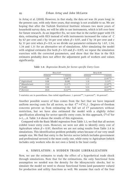
- Page 61: 44Erhan Artuç and John McLarenassu
- Page 65 and 66: 48Erhan Artuç and John McLarenavai
- Page 67 and 68: 50Erhan Artuç and John McLarencomp
- Page 69 and 70: 52Erhan Artuç and John McLarenFigu
- Page 71 and 72: 54Erhan Artuç and John McLarenFigu
- Page 73 and 74: 56Erhan Artuç and John McLarenFigu
- Page 76 and 77: 4Reallocation and Adjustment in the
- Page 78 and 79: Reallocation and Adjustment in the
- Page 80 and 81: Reallocation and Adjustment in the
- Page 82 and 83: Reallocation and Adjustment in the
- Page 84 and 85: Reallocation and Adjustment in the
- Page 86 and 87: Reallocation and Adjustment in the
- Page 88 and 89: 5Trade Reforms in Natural-Resource-
- Page 90 and 91: Trade Reforms in Natural-Resource-A
- Page 92 and 93: Trade Reforms in Natural-Resource-A
- Page 94 and 95: Trade Reforms in Natural-Resource-A
- Page 96 and 97: Trade Reforms in Natural-Resource-A
- Page 98 and 99: Trade Reforms in Natural-Resource-A
- Page 100 and 101: Trade Reforms in Natural-Resource-A
- Page 102 and 103: Trade Reforms in Natural-Resource-A
- Page 104: Trade Reforms in Natural-Resource-A
- Page 107 and 108: 90Olivier Cadot, Laure Dutoit and M
- Page 109 and 110: 92Olivier Cadot, Laure Dutoit and M
- Page 111 and 112: 94Olivier Cadot, Laure Dutoit and M
- Page 113 and 114:
96Olivier Cadot, Laure Dutoit and M
- Page 115 and 116:
98Olivier Cadot, Laure Dutoit and M
- Page 117 and 118:
100Olivier Cadot, Laure Dutoit and
- Page 120 and 121:
7Trade Reform, Employment Allocatio
- Page 122 and 123:
Trade Reform, Employment Allocation
- Page 124 and 125:
Trade Reform, Employment Allocation
- Page 126 and 127:
Trade Reform, Employment Allocation
- Page 128 and 129:
Trade Reform, Employment Allocation
- Page 130 and 131:
Trade Reform, Employment Allocation
- Page 132 and 133:
Trade Reform, Employment Allocation
- Page 134 and 135:
Trade Reform, Employment Allocation
- Page 136 and 137:
Trade Reform, Employment Allocation
- Page 138 and 139:
Trade Reform, Employment Allocation
- Page 140 and 141:
Trade Reform, Employment Allocation
- Page 142 and 143:
Trade Reform, Employment Allocation
- Page 144 and 145:
Trade Reform, Employment Allocation
- Page 146 and 147:
Trade Reform, Employment Allocation
- Page 148 and 149:
Trade Reform, Employment Allocation
- Page 150 and 151:
Trade Reform, Employment Allocation
- Page 152 and 153:
Trade Reform, Employment Allocation
- Page 154 and 155:
Trade Reform, Employment Allocation
- Page 156 and 157:
Trade Reform, Employment Allocation
- Page 158:
Trade Reform, Employment Allocation
- Page 161 and 162:
144Gordon H HansonOn the theory sid
- Page 163 and 164:
146Gordon H Hansonberg et al. (2008
- Page 165 and 166:
148Gordon H HansonThe expansion of
- Page 167 and 168:
150Gordon H Hansonshares and factor
- Page 169 and 170:
152Gordon H HansonGoldberg, Pinelop
- Page 172 and 173:
9Production Offshoring andLabor Mar
- Page 174 and 175:
Production Offshoring and Labor Mar
- Page 176 and 177:
Production Offshoring and Labor Mar
- Page 178 and 179:
Production Offshoring and Labor Mar
- Page 180 and 181:
Production Offshoring and Labor Mar
- Page 182 and 183:
Production Offshoring and Labor Mar
- Page 184 and 185:
Production Offshoring and Labor Mar
- Page 186:
Production Offshoring and Labor Mar
- Page 189 and 190:
172Pravin Krishna and Mine Zeynep S
- Page 191 and 192:
174Pravin Krishna and Mine Zeynep S
- Page 193 and 194:
176Pravin Krishna and Mine Zeynep S
- Page 196 and 197:
11Trade, Child Labor, and Schooling
- Page 198 and 199:
Trade, Child Labor, and Schooling i
- Page 200 and 201:
Trade, Child Labor, and Schooling i
- Page 202 and 203:
Trade, Child Labor, and Schooling i
- Page 204 and 205:
Trade, Child Labor, and Schooling i
- Page 206 and 207:
Trade, Child Labor, and Schooling i
- Page 208 and 209:
Trade, Child Labor, and Schooling i
- Page 210 and 211:
Trade, Child Labor, and Schooling i
- Page 212:
Trade, Child Labor, and Schooling i
- Page 215 and 216:
198Gordon H Hanson3.0%2.8%2.6%2.4%2
- Page 217 and 218:
200Gordon H HansonTable 12.2: Share
- Page 219 and 220:
202Gordon H HansonWho benefits from
- Page 221 and 222:
204Gordon H HansonAn older and larg
- Page 223 and 224:
206Gordon H HansonTo date, the lite
- Page 225 and 226:
208Gordon H Hansontion surplus was
- Page 227 and 228:
210Gordon H HansonSome evidence sug
- Page 229 and 230:
212Gordon H HansonBIBLIOGRAPHYAcost
- Page 231 and 232:
214Gordon H HansonMishra, Prachi 20
- Page 233 and 234:
216James Harrigan• China had been
- Page 235 and 236:
218James Harrigan2.2 Price and quan
- Page 237 and 238:
220James HarriganFigure 13.1a: Pric
- Page 239 and 240:
222James Harrigan4. CONCLUSIONThe e
- Page 241 and 242:
224Beata S Javorcikices, thus benef
- Page 243 and 244:
226Beata S Javorcikfor plants which
- Page 245 and 246:
228Beata S JavorcikAs the majority
- Page 247 and 248:
230Beata S Javorcik5. DOES FDI LEAD
- Page 249 and 250:
232Beata S Javorcikthough they do n
- Page 251 and 252:
234Beata S Javorcik7. FUTURE RESEAR
- Page 253 and 254:
236Beata S JavorcikMarkusen, James
- Page 255 and 256:
238Chad P Bownthese theories has on
- Page 257 and 258:
240Chad P Bownicy changes affect th
- Page 259 and 260:
242Chad P Bownis, the policy-imposi
- Page 261 and 262:
244Chad P Bownsignificant distortio
- Page 263 and 264:
246Chad P Bownaccession period led
- Page 265 and 266:
248Chad P Bown2002-03. 16 However,
- Page 267 and 268:
250Chad P Bowntive adjustment impac
- Page 270:
PART CFACTORS THATAFFECT TRADE
- Page 273 and 274:
256David Hummelsative advantage for
- Page 275 and 276:
258David Hummelsprices shift demand
- Page 277 and 278:
260David HummelsThe second form of
- Page 279 and 280:
262David Hummelsdogenous to how pro
- Page 282 and 283:
17The Duration of Trade Relationshi
- Page 284 and 285:
The Duration of Trade Relationships
- Page 286 and 287:
The Duration of Trade Relationships
- Page 288 and 289:
The Duration of Trade Relationships
- Page 290 and 291:
The Duration of Trade Relationships
- Page 292 and 293:
The Duration of Trade Relationships
- Page 294 and 295:
The Duration of Trade Relationships
- Page 296 and 297:
The Duration of Trade Relationships
- Page 298 and 299:
The Duration of Trade Relationships
- Page 300 and 301:
18Openness and Export Dynamics:New
- Page 302 and 303:
Openness and Export Dynamics: New r
- Page 304 and 305:
Openness and Export Dynamics: New r
- Page 306 and 307:
Openness and Export Dynamics: New r
- Page 308 and 309:
Openness and Export Dynamics: New r
- Page 310 and 311:
19Market Penetration Costs andInter
- Page 312 and 313:
Market Penetration Cost and Interna
- Page 314 and 315:
Market Penetration Cost and Interna
- Page 316 and 317:
Market Penetration Cost and Interna
- Page 318 and 319:
Market Penetration Cost and Interna
- Page 320 and 321:
20Taking Advantage of Trade:The rol
- Page 322 and 323:
Taking Advantage of Trade: The role
- Page 324 and 325:
Taking Advantage of Trade: The role
- Page 326 and 327:
Taking Advantage of Trade: The role
- Page 328 and 329:
Taking Advantage of Trade: The role
- Page 330 and 331:
Taking Advantage of Trade: The role
- Page 332 and 333:
21Credit Constraints and the Adjust
- Page 334 and 335:
Credit Constraints and the Adjustme
- Page 336 and 337:
Credit Constraints and the Adjustme
- Page 338 and 339:
Credit Constraints and the Adjustme
- Page 340 and 341:
Credit Constraints and the Adjustme
- Page 342 and 343:
Credit Constraints and the Adjustme
- Page 344 and 345:
Credit Constraints and the Adjustme
- Page 346:
Credit Constraints and the Adjustme
- Page 349 and 350:
332Miet Maertens and Jo Swinnenmeas
- Page 351 and 352:
334Miet Maertens and Jo Swinnenverg
- Page 353 and 354:
336Miet Maertens and Jo Swinnenacti
- Page 355 and 356:
338Miet Maertens and Jo Swinnenfirm
- Page 357 and 358:
340Miet Maertens and Jo SwinnenBIBL
- Page 359 and 360:
342Miet Maertens and Jo SwinnenRear
- Page 362 and 363:
23Notes on American Adjustment Poli
- Page 364 and 365:
Notes on American Adjustment Polici
- Page 366 and 367:
Notes on American Adjustment Polici
- Page 368 and 369:
Notes on American Adjustment Polici
- Page 370 and 371:
Notes on American Adjustment Polici
- Page 372 and 373:
Notes on American Adjustment Polici
- Page 374 and 375:
Notes on American Adjustment Polici
- Page 376:
Notes on American Adjustment Polici
- Page 379 and 380:
362Johan F M Swinnen and Kristine V
- Page 381 and 382:
364Johan F M Swinnen and Kristine V
- Page 383 and 384:
366Johan F M Swinnen and Kristine V
- Page 385 and 386:
368Johan F M Swinnen and Kristine V
- Page 387 and 388:
370Johan F M Swinnen and Kristine V
- Page 389 and 390:
372Johan F M Swinnen and Kristine V
- Page 391 and 392:
374Johan F M Swinnen and Kristine V
- Page 393 and 394:
376Johan F M Swinnen and Kristine V
- Page 395 and 396:
378Johan F M Swinnen and Kristine V
- Page 397 and 398:
380Johan F M Swinnen and Kristine V
- Page 399:
This book summarizes the state of k