Métodos numericos: ecuaciones diferenciales ordinarias

Métodosdeunpaso
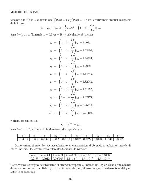
tenemos que f(t, y) =y, porloque ∂f
∂f
(t, y) =0y (t, y) =1, y así la recurrencia anterior se expresa
∂t ∂y
de la forma
yi = yi−1 + yi−1h + 1
2 yi−1h 2 µ
= 1+h + h2
yi−1,
2
para i =1, ..., n. Tomando h =0.1 (n =10) y calculando obtenemos
µ
y1 = 1+h + h2
y0 =1.105,
2
µ
y2 = 1+h + h2
y1 =1.22103,
2
µ
y3 = 1+h + h2
y2 =1.34923,
2
µ
y4 = 1+h + h2
y3 =1.4909,
2
µ
y5 = 1+h + h2
y4 =1.64745,
2
µ
y6 = 1+h + h2
y5 =1.82043,
2
µ
y7 = 1+h + h2
y6 =2.01157,
2
µ
y8 = 1+h + h2
y7 =2.22279,
2
µ
y9 = 1+h + h2
y8 =2.45618,
2
µ
y10 = 1+h + h2
y9 =2.71408,
2
y ahora los errores son
ei = |e i∗0.1 − yi|,
para i =1, ..., 10, que nos da la siguiente tabla aproximada
e1 e2 e3 e4 e5 e6 e7 e8 e9 e10
0.00017 0.0004 0.0006 0.0009 0.0013 0.0017 0.0022 0.0028 0.0034 0.0042
Como vemos, el error decrece notablemente en comparación al obtenido al aplicar el método de
Euler. Además, los errores para diferentes tamaños de paso son
h =1 h =0.1 h =0.01 h =0.001 h =0.0001 h =0.00001
0.2183 0.0042 0.000045 4.5 · 10 −7 4.5 · 10 −9 4.5 · 10 −11
Como vemos, se mejora notablemente el error con respecto al método de Taylor, siendo éste además
de orden dos, es decir, al dividir por 10 el tamaño de paso, el error es aproximadamente el del paso
anterior al cuadrado.
28