Métodos numericos: ecuaciones diferenciales ordinarias
Métodos numericos: ecuaciones diferenciales ordinarias
Métodos numericos: ecuaciones diferenciales ordinarias

You also want an ePaper? Increase the reach of your titles
YUMPU automatically turns print PDFs into web optimized ePapers that Google loves.
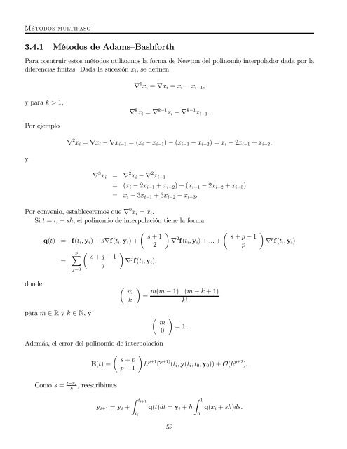
<strong>Métodos</strong> multipaso<br />
3.4.1 <strong>Métodos</strong> de Adams—Bashforth<br />
Para cosntruir estos métodos utilizamos la forma de Newton del polinomio interpolador dada por la<br />
diferencias finitas. Dada la sucesión xi, sedefinen<br />
yparak>1,<br />
Por ejemplo<br />
y<br />
∇ 1 xi = ∇xi = xi − xi−1,<br />
∇ k xi = ∇ k−1 xi −∇ k−1 xi−1.<br />
∇ 2 xi = ∇xi −∇xi−1 =(xi − xi−1) − (xi−1 − xi−2) =xi − 2xi−1 + xi−2,<br />
∇ 3 xi = ∇ 2 xi −∇ 2 xi−1<br />
= (xi−2xi−1 + xi−2) − (xi−1 − 2xi−2 + xi−3)<br />
= xi − 3xi−1 +3xi−2 − xi−3.<br />
Por convenio, estableceremos que ∇ 0 xi = xi.<br />
Si t = ti + sh, el polinomio de interpolación tiene la forma<br />
µ<br />
s +1<br />
q(t) = f(ti, yi)+s∇f(ti, yi)+<br />
2<br />
pX<br />
µ <br />
s + j − 1<br />
=<br />
∇<br />
j<br />
j f(ti, yi),<br />
j=0<br />
donde µ m<br />
k<br />
para m ∈ R y k ∈ N, y<br />
<br />
= m(m − 1)...(m − k +1)<br />
<br />
∇ 2 µ<br />
s + p − 1<br />
f(ti, yi)+... +<br />
p<br />
k!<br />
µ m<br />
0<br />
Además, el error del polinomio de interpolación<br />
E(t) =<br />
Como s = t−xi , reescribimos<br />
h<br />
µ s + p<br />
p +1<br />
yi+1 = yi +<br />
<br />
=1.<br />
<br />
h p+1 f p+1) (ti, y(ti; t0, y0)) + O(h p+2 ).<br />
Z ti+1<br />
ti<br />
q(t)dt = yi + h<br />
52<br />
Z 1<br />
0<br />
q(xi + sh)ds.<br />
<br />
∇ p f(ti, yi)