Métodos numericos: ecuaciones diferenciales ordinarias

El método de Adams—Bashforth se construye a partir del desarrollo
Z 1
yi+1 = yi + h
0
q(xi + sh)ds
ÃZ 1 pX
µ
s + j − 1
= yi + h
∇
0
j
j=0
j !
f(ti, yi)ds
Ã
pX
= yi + h ∇ j Z 1 µ !
s + j − 1
f(ti, yi)
ds
j
= yi + h
j=0
pX
γj∇ j f(ti, yi),
donde los coeficientes
γ0 = 1,
Z 1 µ
s + j − 1
γj =
ds, j =1, 2, ..., p,
0 j
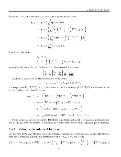
se calculan de forma directa. De hecho, los primeros coeficientes son
j=0
γ 1 γ 2 γ 3 γ 4 γ 5 γ 6
1
2
5
12
3
8
251
720
0
95
288
Además, el error local de truncamiento es de la forma
19087
60480
ti+1 = −h p+2 γ p+1y p+2 (ti; t0, y0)+O(h p+3 ),
Métodos multipaso
por lo que es orden O(hp+2 ). Así, si buscamos un método de error global O(h3 ), necesitaremos que
p =2,siendoelmétododelaforma
µ
yi+1 = yi + h f(ti, yi)+ 1
2 ∇f(ti, yi)+ 5
12 ∇2
f(ti, yi)
µ
= yi + h f(ti, yi)+ 1
2 [f(ti, yi)+f(ti−1, yi−1)]
+ 5
12 [f(ti,
yi) − 2f(ti−1, yi−1)+f(ti−2, yi−2)]
= yi + 1
12 h (23f(ti, yi) − 16f(ti−1, yi−1)+5f(ti−2, yi−2)) .
Como vemos, al método de Adams—Bashforth le podemos aplicar el teorema de convergencia global,
por lo que será convergente, al contrario de lo que ocurría con el primer ejemplo que estudiamos.
3.4.2 Métodos de Adams—Moulton
Los métodos de Adams—Moulton se obtienen de igual manera que los explícitos de Adams—Basfhforth,
pero ahora tomando el polinomio interpolador en t = ti+1 + sh, conloque
q ∗ µ
s +1
(t) = f(ti+1, yi+1)+s∇f(ti+1, yi+1)+ ∇
2
2 µ
s + p − 1
f(ti, yi)+... +
p
53
∇ p f(ti+1, yi+1)