Fisheries in the Southern Border Zone of Takamanda - Impact ...

More documents

Recommendations

Info

174 Slayback 7 H S IH type of automated change detection methods used (a composite multi-date classification; more below), atmospheric correction was not required (Song, Woodcock et al. 2001). The full Landsat scenes were subset to a 1600 x 1760 pixel (~46 x 50 km) window surrounding the TFR (Photo gallery). The Landsat TM instrument records imagery at 30meter resolution in 6 different spectral bands, including 3 bands in the visible and 3 in the infrared. Vegetation is known to respond strongly in the red and infrared bands; healthy green leaf matter absorbs red radiation and strongly reflects near-infrared. Additionally, Boyd and Duane (2001) found that the green (band 2) and middle infrared (bands 5 and 7) wavelengths are useful in discriminating tropical forest regeneration. In humid tropical environments, imagery in the blue wavelengths Takamanda: the Biodiversity of an African Rainforest 7 e˜2p 7 y2@w—˜A 7 e—22S22 —22I222— †— g2‚ g2‚ g2‚ g2‚ g2‚ g2‚ g2‚ g2‚ g2‚ g2‚ g2‚ g2‚ g2‚ g2‚ g2‚ g2‚ g2‚ g2‚ g2‚ g2‚ g2‚ g2‚ g2‚ g2‚ g2‚ x——2€— x——2€— x——2€— x——2€— x——2€— x——2€— x——2€— x——2€— x——2€— x——2€— x——2€— x——2€— x——2€— x——2€— x——2€— x——2€— x——2€— x——2€— x——2€— x——2€— x——2€— x——2€— x——2€— x——2€— x——2€— y—2h y—2h y—2h y—2h y—2h y—2h y—2h y—2h y—2h y—2h y—2h y—2h y—2h y—2h y—2h y—2h y—2h y—2h y—2h y—2h y—2h y—2h y—2h y—2h y—2h 7 u 7 7 7 7 w— 7 7 7 7 w— 7 7 7 7 „———— „———— „———— „———— „———— „———— „———— „———— „———— „———— „———— „———— „———— „———— „———— „———— „———— „———— „———— „———— „———— „———— „———— „———— „———— p p p p p p p p p p p p p p p p p p p p p p p p p ‚ ‚ ‚ ‚ ‚ ‚ ‚ ‚ ‚ ‚ ‚ ‚ ‚ ‚ ‚ ‚ ‚ ‚ ‚ ‚ ‚ ‚ ‚ ‚ ‚ 7 7 w—— 7 7 (band 1) is generally dominated by scattering off of water vapor particles, and so appears very hazy, and relatively little useful ground-reflected signal penetrates this haze. Thus, I used the green (band 2), red (band 3), near infrared (band 4) and middle infrared (bands 5 and 7) bands for this analysis. 2.2 Change classification 7 7 7 7 7 7 7 7 7 7 7 7 Changes in landcover between the two dates of imagery were estimated using standard supervised classification techniques. Specifically, the maximum likelihood algorithm method was used in PCI’s Imageworks software package. This method assigns class membership based on the statistical properties (mean and standard deviation) of each defined class for all included image bands. 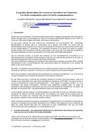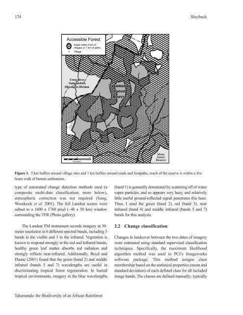The classes are defined manually; typically 7 7 7 7 7 7 7 w p ‚ Figure 1. 5 km buffers around village sites and 1 km buffers around roads and footpaths; much of the reserve is within a few hours walk of human settlements. 7
Landcover change an operator with knowledge of the imagery manually delineates sites (groups of pixels) of each class on the imagery. Based on the spectral character of these training sites, the maximum likelihood algorithm then makes probability-based class assignments of all image pixels. To generate landcover change classes using these classification methods, the training sites were selected to include both change classes (such as “forest to nonforest”) and non-change classes (“unchanged lowland forest”), and the spectral bands from both dates of imagery were input to the classification procedure simultaneously. This is sometimes termed composite multi-date classification, since images from both dates are composited and used together, as if from a single date. The preliminary orthorectification step makes this approach possible as it ensures the precise overlay of images from different dates. After running the classification, some post-classification processing and manual editing were conducted to clean up and finalize the classification map. Various statistics were calculated from this final classification map to quantify changes in landcover. To provide better insight into where changes might be occurring most rapidly, these measures were calculated for several regions: the entire 1600 x 1740 image subset; the area within the TFR boundaries (excluding enclave communities); the areas of the two enclave communities (Obonyi and Kekpane); and the area within a 5-km buffer zone surrounding the TFR. 3 Results 3.1 Change Classification Training sites for nine different classes were initially defined (see Sunderland et al. this volume) to include eight static classes (lowland forest, ridge forest, midelevation forest, montane forest, grassland/bare, secondary forest/farms, water, shadow), and one change class indicating forest conversion (forest → secondary forest/farms). Note that in a static interpretation of the output classification (e.g. for a year 2000 landcover map), the forest conversion class would be added to the secondary forest/farms class. No distinction was made 175 between secondary forest and farms because these two landcover types are fluid and difficult to distinguish; farms usually have a scattering, or more, of larger trees, and due to the agricultural practices in the region, areas of secondary forest will be farmed again after several years of forest regrowth. The four different types of undisturbed forest (lowland, ridge, mid-elevation, and montane) were included in the classification both because we wanted to map the extent of these forest types (see Sunderland et al. this volume), and because lumping them together produces an overly broad and poorly defined forest class, which becomes confused with secondary forest in the classification results. Several other types of change might have also been included, but were not, such as grassland → burned grassland, and forest regrowth (farms → secondary forest); these were either not of interest (the former) or too difficult to consistently differentiate (the latter). In either case, we verified that these areas were satisfactorily classified with the existing scheme. For example, the grassland → burned grassland areas were routinely classified as grassland, and the areas of possible regrowth (farms → secondary forest) were classified as secondary forest. A class for shadow was necessary because the poor and variable illumination on the shadowed sides of hills makes differentiation of different landcovers much more difficult. The resulting classification was then visually inspected, and in an iterative process, minor adjustments were made to the training classes and certain classification parameters. Despite many such adjustments, it became apparent that an additional class would be useful to indicate areas of “possible” secondary forest. These areas can typically be classified as either lowland forest, secondary forest, or ridge forest, depending on the set of training sites and classification parameters. However, as these areas do not appear to be separable solely from image reflectances, it was decided to create a separate “possible secondary forest” (PSF) class. Generally, firsthand knowledge of the area is required to assign definitive labels to these regions, but many can be labeled based on a closer inspection of the imagery; for example, the areas on hillsides not in the vicinity of villages are most likely undisturbed forest SI/MAB Series #8, 2003
Page 2 and 3:
Smithsonian Institution SI/MAB Biod
Page 4 and 5:
ii 10. Fisheries in the Southern Bo
Page 6 and 7:
Mercy Abwe Dione Dept. of Biology,
Page 8 and 9:
The Smithsonian Institution has lon
Page 10 and 11:
The editors of this publication ext
Page 12 and 13:
2 Sunderland-Groves et al. Figure 1
Page 14 and 15:
4 Sunderland-Groves et al. Rainfall
Page 16 and 17:
6 Sunderland-Groves et al. 7 Conser
Page 18 and 19:
8 Sunderland-Groves et al. Europe,
Page 20 and 21:
10 Comiskey and Dallmeier 2 Challen
Page 22 and 23:
12 Comiskey and Dallmeier 5 Adaptiv
Page 24 and 25:
14 Comiskey and Dallmeier identifie
Page 26 and 27:
16 Comiskey and Dallmeier 5.4 Evalu
Page 28 and 29:
18 Takamanda: the Biodiversity of a
Page 30 and 31:
20 Sunderland et al. preliminary la
Page 32 and 33:
22 Sunderland et al. avoided protru
Page 34 and 35:
24 Sunderland et al. Table 2. Summa
Page 36 and 37:
26 Sunderland et al. lowland forest
Page 38 and 39:
28 Sunderland et al. impressive cat
Page 40 and 41:
30 Sunderland et al. Herbaceous flo
Page 42 and 43:
32 Sunderland et al. Table 3. Compa
Page 44 and 45:
34 Sunderland et al. 5.5 Economic P
Page 46 and 47:
36 Sunderland et al. Table 5. Summa
Page 48 and 49:
38 Sunderland et al. monitoring pro
Page 50 and 51:
40 Sunderland et al. Letouzey, R. 1
Page 52 and 53:
42 Sunderland et al. Appendix 1. Pl
Page 54 and 55:
44 Sunderland et al. Agelaea pentag
Page 56 and 57:
46 Sunderland et al. Afzelia pachyl
Page 58 and 59:
48 Sunderland et al. Rhabdophyllum
Page 60 and 61:
50 Sunderland et al. Aningeria robu
Page 62 and 63:
52 Sunderland et al. Nervilia sp. P
Page 64 and 65:
54 Sunderland et al. g—2˜— @y
Page 66 and 67:
56 O’Kah f22 y2@w—˜A g—22@IE
Page 68 and 69:
58 O’Kah Table 3. Species found i
Page 70 and 71:
60 O’Kah Table 6. Indicators of s
Page 72 and 73:
62 O’Kah Larsen, T. B. 1997. Butt
Page 74 and 75:
64 O’Kah Appendix 1 (cont.). Chec
Page 76 and 77:
66 O’Kah Appendix 1 (cont.). Chec
Page 78 and 79:
68 O’Kah Species distribution Tak
Page 80 and 81:
70 O’Kah Species distribution Tak
Page 82 and 83:
72 Takamanda: the Biodiversity of a
Page 84 and 85:
74 h—2@y——A 2 IE2— y2@w—
Page 86 and 87:
76 The sites which have been survey
Page 88 and 89:
78 species from a phylogenetic poin
Page 90 and 91:
80 Appendix 1. Species list and sam
Page 92 and 93:
82 Family / Species Notes Locations
Page 94 and 95:
84 LeBreton et al. 3 Methods A team
Page 96 and 97:
86 LeBreton et al. Bothrolycus ater
Page 98 and 99:
88 LeBreton et al. an important par
Page 100 and 101:
90 LeBreton et al. Perret, J.-L. 19
Page 102 and 103:
92 LeBreton et al. Appendix 1 (cont
Page 104 and 105:
94 LeBreton et al. Appendix 1 (cont
Page 106 and 107:
96 Languy and Motombe f 5 q—2˜
Page 108 and 109:
98 Languy and Motombe Table 3. Thre
Page 110 and 111:
100 Languy and Motombe encroachment
Page 112 and 113:
102 Languy and Motombe Appendix 1.
Page 114 and 115:
104 Languy and Motombe Appendix 1 (
Page 116 and 117:
Page 118 and 119:
Page 120 and 121:
Page 122 and 123:
112 Sunderland-Groves and Maisels h
Page 124 and 125:
114 Sunderland-Groves and Maisels T
Page 126 and 127:
116 Sunderland-Groves and Maisels T
Page 128 and 129:
118 Sunderland-Groves and Maisels B
Page 130 and 131:
120 Sunderland-Groves and Maisels S
Page 132 and 133:
122 Sunderland-Groves and Maisels A
Page 134 and 135: 124 Sunderland-Groves and Maisels A
Page 136 and 137: 126 Sunderland-Groves and Maisels A
Page 138 and 139: 128 Takamanda: the Biodiversity of
Page 140 and 141: 130 Sunderland-Groves et al. In mor
Page 142 and 143: 132 Sunderland-Groves et al. proved
Page 144 and 145: 134 Sunderland-Groves et al. q—2
Page 146 and 147: 136 Sunderland-Groves et al. Table
Page 148 and 149: 138 Sunderland-Groves et al. from m
Page 150 and 151: 140 Sunderland-Groves et al. Sander
Page 152 and 153: 142 Mdaihli et al. Basin and is sep
Page 154 and 155: 144 Table 1. Type and number of fis
Page 156 and 157: 146 Migrating Labeo spp. make up 10
Page 158 and 159: 148 Mdaihli et al. Mochokidae Barbu
Page 160 and 161: 150 Monthly yield (t) 200 160 120 8
Page 162 and 163: 152 Mdaihli et al. of Forests Aroun
Page 164 and 165: 154 Mdaihli et al. Appendix 1 (cont
Page 166 and 167: 156 Sunderland et al. Table 1. Majo
Page 168 and 169: 158 Sunderland et al. resources and
Page 170 and 171: 160 Sunderland et al. No. of indivi
Page 172 and 173: No. of individuals (n = 315) 200 15
Page 174 and 175: No. of individuals (n = 1065) 1000
Page 176 and 177: Gnetum spp. Piper guineensis Site T
Page 178 and 179: Resource Impacts of seasonality Ava
Page 180 and 181: Box. Large-scale exploitation of no
Page 182 and 183: Sunderland, T. C. H. 2001. Cross Ri
Page 186 and 187: 176 Slayback (ridge or lowland). On
Page 188 and 189: 178 Slayback Table 2: Areas of outp
Page 190 and 191: 180 Takamanda: the Biodiversity of
Page 192: 182 Sunderland-Groves et al. Mone F
show all

Fisheries in the Southern Border Zone of Takamanda - Impact ...

You also want an ePaper? Increase the reach of your titles

Delete template?

Save as template?