The international economics of resources and resource ... - Index of
The international economics of resources and resource ... - Index of
The international economics of resources and resource ... - Index of

Create successful ePaper yourself
Turn your PDF publications into a flip-book with our unique Google optimized e-Paper software.
Sustainability <strong>economics</strong>, <strong>resource</strong> efficiency, <strong>and</strong> the Green New Deal 195<br />
Moreover, we assume for simplicity in the medium-run analysis that the<br />
production technologies <strong>of</strong> Y <strong>and</strong> K are symmetric <strong>and</strong> <strong>of</strong> the Cobb-Douglas<br />
form. In this way, (3) can be simplified <strong>and</strong> K accumulates according to:<br />
where s is the savings rate. A(t) now reads:<br />
¨K(t) η<br />
A(t) = Ã<br />
Z (t) 1−α<br />
˙K(t) = s · Y(t) − δK(t) (15)<br />
(16)<br />
where ¨K is actually used capital ( ¨K < K when BK < DE) <strong>and</strong> we again divide<br />
by Z 1−α to eliminate the scale effect. During a cycle, maximum output is<br />
obtained with B(t) · K(t) = D(t) · E(t), which applies when energy supply is<br />
fully elastic. <strong>The</strong>n, the model predicts cyclical energy use.<br />
Regarding the supply <strong>of</strong> energy we argue along two possible scenarios. In<br />
regime 1 (“affluent energy”), energy supply is fully elastic at given energy<br />
prices ¯pE:<br />
pE = ¯pE<br />
(17)<br />
Growth in regime 1 is then determined by BK = DE, ˜K = BK, <strong>and</strong> ¨K = K<br />
so that we obtain:<br />
Y = ÃB α K α+η<br />
(18)<br />
ˆK = sÃB α K α+η−1 − δ (19)<br />
In regime 2 (“limiting energy”), energy supply is restricted according to:<br />
E = Ē < B · K/D (20)<br />
Growth in regime 2 is thus bounded by energy supply Ē.<br />
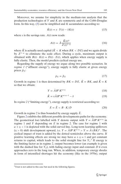
Figure 2 exhibits the different possible developments paths for the economy.<br />
<strong>The</strong> geometrical loci labelled with Y denote output with Y = ÃB α K α+η in<br />
regime 1 <strong>and</strong> Y depending on E in regime 2. <strong>The</strong> case for regime 1 with<br />
α + η0) shift development upward, i.e. Y = ÃB α K α+η > Y = Ã (BK) α . <strong>The</strong><br />
cyclical impact <strong>of</strong> trust is added by the dotted semicircles above the curve. If<br />
positive learning effects are strong we may have α + η = 1 <strong>and</strong> get constant<br />
returns to capital, which leads to the solid straight line for Ys. 5 If energy is<br />
the limiting factor as in regime 2, output becomes lower (an example is given<br />
with the dashed line for Yd), with fading energy input <strong>and</strong> constant D it even<br />
approaches zero in the long run. When, in addition, temporary energy shocks<br />
in form <strong>of</strong> intensified shortages hit the economy (like in the 1970s), output<br />
5 Trust is not added in this case but used in the following figures.