Phase-field modeling of diffusion controlled phase ... - KTH Mechanics

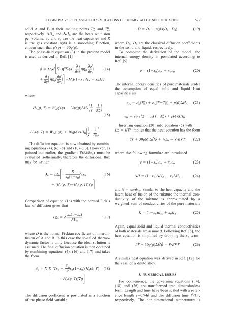
LOGINOVA et al.: PHASE-FIELD SIMULATIONS OF BINARY ALLOY SOLIDIFICATION575solid A and B at their melting points T A m and T B m,respectively. H A and H B are the heats of fusionper volume, c A and c B are the heat capacities and Ris the gas constant. p(f) is a smoothing function,chosen such that p(f) 30g(f).The phase-field equation (3) in the present modelis used as derived in Ref. [1]whereḟ M f ¯2·(h 2 f)∂xhh ∂ b ∂f (14)∂y∂yhh ∂ b ∂f∂xM f ((1x B )H A x B H B )H A (f, T) W A g(f) 30g(f)H A 1 T 1T A m(15)H B (f, T) W B g(f) 30g(f)H B 1 T 1T B mThe diffusion equation is now obtained by combiningequations (4), (6), (8) and (10)–(13). However, aspointed out earlier, the gradient (δS/δx B ) must beevaluated isothermally, therefore the diffusional fluxmay be writtenJ B L A BBRx B (1x B ) x B (16) (H A (f, T)H B (f, T))fComparison of equation (16) with the normal Fick’slaw of diffusion gives thatL A BB D x B(1x B )RV m(17)where D is the normal Fickian coefficient of interdiffusionof A and B. In this case the so-called thermodynamicfactor is unity because the ideal solution isassumed. The final diffusion equation is then obtainedby combining equations (4), (16) and (17) and takesthe formẋ B ·Dx B V mR x B(1x B )(H B (f, T) (18)H A (f, T))fThe diffusion coefficient is postulated as a functionof the phase-field variableD D S p(f)(D L D S ) (19)where D S , D L are the classical diffusion coefficientsin the solid and liquid, respectively.To complete the derivation of the model, theinternal energy density is postulated according toRef. [5]e (1x B )e A x B e B (20)The internal energy densities of pure materials underthe assumption of equal solid and liquid heatcapacities aree A e s A(T A m) c A (TT A m) p(f)H A (21)e B e s B(T B m) c B (TT B m) p(f)H BInserting equation (20) into equation (5) withL A ee KT 2 implies that the heat equation has the formc¯Ṫ 30g(f)H˜ ḟ Nẋ B ·KT (22)where the following formulae are introducedc˜ (1x B )c A x B c B (23)H˜ (1x B )H A x B H B (24)and N ∂e/∂x B . Similar to the heat capacity and thelatent heat of fusion of the mixture the thermal conductivityof the mixture is approximated by aweighted sum of conductivities of the pure materialsK (1x B )K A x B K B (25)Again, equal solid and liquid thermal conductivitiesof both materials are assumed. Following Ref. [8], theheat equation is simplified by dropping the ẋ B termc¯Ṫ 30g(f)H˜ ḟ ·KT (26)A similar heat equation was derived in Ref. [12] forthe case of a dilute alloy.3. NUMERICAL ISSUESFor convenience, the governing equations (14),(18) and (26) are transformed into dimensionlessform. Length and time have been scaled with a referencelength l0.94d and the diffusion time l 2 /D L ,respectively. The non-dimensional temperature is