Phase-field modeling of diffusion controlled phase ... - KTH Mechanics

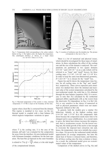
578 LOGINOVA et al.: PHASE-FIELD SIMULATIONS OF BINARY ALLOY SOLIDIFICATIONFig. 3. Temperature field corresponding to the solute redistributionin Fig. 2. The lighter color, the higher the temperature.The solid/liquid interface is shown as a band where0.1f0.9. Time is 2.75 ms.Fig. 4. Maximal temperature of the system vs time, minimaltemperature T1574K is kept on the boundary all the time.regime when a heat flux is extracted from the domain.This regime is modeled in two ways: (a) the isothermalmodel is coupled with a heat balance [4]which neglects temperature variations in spacedTdtṪ H˜c˜ddt 1 f(x, y, t)dS (30)SSwhere Ṫ is the cooling rate, S is the area of thedomain, H˜ and c˜ are evaluated for the compositionfar away from the interface; (b) non-isothermal modelwith Neumann boundary conditions for the heat equation.The heat flux Q imposed on the outer boundaryis related to Ṫ by Q c˜Ṫa , where a is the side length4of the computational domain.Fig. 5. Location of isotherms near the dendrite tip. The picturecorresponds to the run in Fig. 3.There is a lot of numerical and physical issues,which should be investigated for these types of simulations.In these calculations the effect of the coolingrate and the size of the domain is analyzed. The computationsare performed in two square domains6.910 5 and 2.2810 5 m on a side (which will bereferred to as “large” and “small” boxes), for threecooling rates: 2.110 3 , 3.410 4 , and 1.310 5 K/s.In order to keep the same non-dimensional geometry,d1.6210 8 m is chosen for the “small” box.Figure 6(a and b) shows the temperature–time historyfor all cooling rates, in the “big” and “small”box, respectively. Three curves represent each simulation:two dashed lines show the minimal and maximalvalue of the system temperature calculated by thenon-isothermal model, the solid line is T(t) obtainedthrough the heat balance [equation (30)]. It is necessaryto note that T(t) calculated by the isothermalapproach differs significantly (2K as the worst) fromthe short-term T(t) dependence in Fig. 6 in Ref. [4].T(t) is very sensitive to the choice of numerical aswell as physical parameters which were not unambiguouslydefined in Ref. [4].In general, both the models give a similar T(t)behaviour. Initially, at the highest cooling rates(3.410 4 and 1.310 5 K/s) the temperature fallsdown because the composition needs more time to bechanged and to cause solidification. As a crystal startsto grow, the latent heat release increases the temperature,that is, recalescence occurs. For the lowest coolingrate, the initial growth of the nuclei is fast enoughto overcome the imposed heat extraction rate and,hence, the temperature–time curve initially has a positiveslope. T(t) given by the isothermal model initiallyapproximates an average temperature, but later thelatent heat of fusion is released faster, and therefore,for all three cooling rates the time evolution is faster.As a result, the isothermal model gives an overestimatedvalues of the temperature.Comparison of the dashed curves in Fig. 6(a and