Phase-field modeling of diffusion controlled phase ... - KTH Mechanics

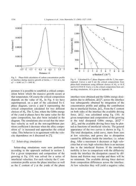
1334 I. Loginova et al. / Acta Materialia 51 (2003) 1327–1339Fig. 3. Phase-field calculation of carbon concentration profileat interface during massive growth of ferrite, v 0.1 m/s, foru gC 0.001 at T = 1093 K.perature it is possible to establish a critical compositionbelow which the massive growth occurs atthat temperature. Of course the critical compositiondepends on the value of M f . In Fig. 4 we havesuperimposed, on a part of the calculated Fe–Cphase diagram, curves a and b representing thecritical composition calculated for two differentchoices of M f . The T 0 line, where the Gibbs energyof the g and a phases have the same value for thesame composition, has also been included in thediagram. The simulations also reveal that the interfacevelocity as well as the non-equilibrium partitioncoefficient k decrease when the alloy compositionu gC is increased and approaches the criticalvalue. This behavior is in agreement with the velocitydependence on k discussed in [7].7.2. Solute-drag simulationsSolute-drag simulations were now performedaccording to the approach outlined in section 3.For a given temperature and composition of thegrowing a Eq. (14) was solved for a series ofinterfacial velocities. For each velocity the C concentrationprofile across the phase interface as wellas the C content of g at the g-side of the phaseFig. 4. Calculated Fe–C phase diagram with the T 0 line superimposed.Curves a and b are the critical compositions fromphase-field simulations using different choices of M f :a)M/dand b) 0.235M/d. Curve c) is the critical composition from solute-dragsimulations. M is given in Appendix B.interface were obtained and the Gibbs energy dissipationdue to diffusion, G diffm , across the interfacewas subsequently obtained by integration of theconcentration profile and adding the contributiondue to interfacial friction, G i m. From the C contenton both sides of the interface the available drivingforce, G totm , was calculated using Eq. (18). Atgiven temperature and composition of the growinga the total dissipated Gibbs energy, G diffm G i m, and the available driving force may be plottedas functions of interfacial velocity. The generalappearance of the two curves is shown in Fig. 5.The total dissipation, solid curve, starts from zeroat low velocities, and grows due to dissipationcaused by diffusion inside the interface, i.e. solutedrag. After a maximum it decreases at high velocitiesbut at very high velocities there is an increasedue to the interfacial friction. If the interfacialmobility is low in comparison with the diffusivityinside the interface the dissipation caused by diffusionand friction may overlap and there will beno minimum. The available driving force derivesfrom composition differences across the interface.At low velocities they will yield a negative value