Phase-field modeling of diffusion controlled phase ... - KTH Mechanics

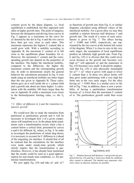
1336 I. Loginova et al. / Acta Materialia 51 (2003) 1327–1339contents given by the phase diagram, i.e. localequilibrium is established, but they approach eachother at higher growth rates. The point of tangencybetween the dissipation and driving force curves inFig. 5 appears as a maximum on the curve foru a C denoted by the dot in Fig. 6 and the two curveshave then got very close to each other. Thismaximum represents the highest C content that acould grow with. With a mobility according toAppendix B, the maximum C content of a fellclose to the equilibrium phase boundary for a.However, the maximum C content and the correspondinggrowth rate depend on the properties ofthe interface. The higher the interfacial mobility,compared to the diffusivity, the higher themaximum content and the corresponding growthrate. In order to demonstrate clearly the generalbehavior the calculations presented in Fig. 6 weremade using an interfacial mobility ten times largerthan the one given in Appendix B. These calculationsgave an a well inside the a + g phase fieldand a growth rate about ten times higher. A calculationwith the mobility 100 times larger than theone in Appendix B yields a maximum even closerto the thermodynamic limiting value, i.e. the T 0line.as functions of growth rate from Fig. 6, or similardiagrams calculated using different values of theinterfacial mobility. For a given alloy we may thusestablish a relation between half thickness andgrowth rate. The result of a series of such calculationsis given in Fig. 7. The alloys havinguCg 0.008 and 0.005, respectively, are representedby the two curves at the bottom left cornerof the diagram. When is close to zero in the veryearly stages, the assumption of local equilibriumpredicts an infinitely high growth rate. From Fig.6 and Eq. (19) it is obvious that this could neveroccur because as the growth rate becomes veryhigh u g C/a will approach u a C and the numerator inEq. (19) becomes very small. It should be emphasizedthat Eq. (19) is only physically meaningfulfor u g/aC uCg when a grows with equal or lowerC content than g. In these two alloys ferrite willthus grow under partitioning with a very high butfinite rate in the very early stages. For the alloyhaving u gC 0.003 there is a similar curve to theleft in Fig. 7 but, in addition, there is now a possibilityof having a partitionless transformationbecause u gC is lower than the maximum C contentof a. The partitionless growth could then occur7.3. Effect of diffusion in g and the transition tomassive growthWe would now like to study the transition frompartitional to partitionless growth and it will benecessary to investigate how g of a given compositionwill transform to a. In the phase-field simulationssuch a transformation occurs when g has acontent below a critical limit, presented by curvesa and b for different M f values, in Fig. 4. In orderto investigate the predictions of solute drag theoryit is necessary to account for C diffusion in g aheadof the migrating g/a interface. It should first of allbe realized that the calculations for the interfacewere made under steady-state growth, whichstrictly implies that the transformation is partitionless.However, it has already been mentionedthat the results could be used as a good approximationfor non-steady state conditions, i.e. for partitionaltransformations.We now apply Eq. (19) and take u a Cand u g/aCFig. 7. Relation between half thickness and growth rate predictedfrom Eq. (19) and Fig. 6. Each curve holds for a differentalloy content as indicated. The hatched area represents velocitieswhere no physical solutions are possible.