Phase-field modeling of diffusion controlled phase ... - KTH Mechanics

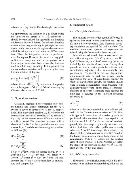
1332 I. Loginova et al. / Acta Materialia 51 (2003) 1327–1339where a (df/dz) 2 dz. For the simple case wheredwe approximate the variation in f as linear insidethe interface we obtain a 1/d. However, itshould be emphasized that generally the interfacethickness is less well defined for a diffuse interfacethan in solute drag modeling. In principle the interfaceextends over the whole region where f varies,which is strictly z for the diffuse interface.Thus, the integration should be performedover that region. However, in practice it may yieldsufficient accuracy to extend the integration over afinite region somewhat thicker than the thicknessused in solute drag modeling. In the present casea more realistic variation in f is given by the equilibriumsolution of Eq. (6):f 1 21 tanhz/2d (30)where d e/√W/V m . By numerical integrationover a the region 3d z 3d and adopting Eq.(30) one obtains a 0.235/d.5. Physical parametersAs already mentioned, the complete set of thermodynamicand kinetic parameters for the Fe–Csystem is given in appendices A and B, respectively.The phase-field mobility M f is related to theconventional interfacial mobility M by means ofEq. (29). In the present study different choices ofa will be tested. The interface thickness will bechosen as d = 10 9 m. For a pure element the parametersW, , d and the surface energy s are relatedas follows [16]:W s d V 6m(31)2Ws e (32)18V mi.e. e 2 3√2sd. With the surface energy s 1J/m 2 and V m 710 6 m 3 mol 1 we obtain W =29.698 10 3 J/mol e 2 4.24 10 9 J/m. We shallassume that W and are independent of temperatureand composition.6. Numerical details6.1. Phase-field simulationsThe standard second order central difference inspace and first order in time transform Eqs. (6) and(7) into a discrete problem. Zero Neumann boundaryconditions are applied for both variables. Theresulting non-linear systems of equations aresolved using the Newton–Raphson method.From the experimental observations, we expecttwo different regimes: “slow” growth, controlledby C diffusion in g, and “fast” massive growth controlledby the interfacial reactions. During slowgrowth, we thus expect a parabolic behavior withan interface velocity v that is essentially proportionalto 1/√t except for the later stages whenimpingement sets in and the system finallyapproaches the state of equilibrium. During the“fast” or partitionless growth, the solution shouldyield a single concentration spike traveling withconstant velocity v until all the initial γ is transformedinto a. In order to simulate these regimes thetime step is adjusted to the interface dynamicsaccording tot ch (33)nwhere h is the space resolution in a uniform gridand c is the Courant number taken as 0.01. Withthis approach simulations of massive growth areperformed with constant time step equal to itsinitial value 3.5· 10 10 s. In the case of parabolicgrowth, the time step is gradually increased andat the final time, when the equilibrium is nearlyachieved, t is 10 6 times larger than initially. Thechoice of the grid resolution was verified based onthe known content of carbon in both phases at theequilibrium. With h 0.1125 nm the relativeerror of equilibrium u C is 1.2%. Another test is thatthe slope of the interface position vs √t is a constantexcept for the later stages.6.2. Solute drag simulationsThe steady-state diffusion equation, i.e. Eq. (14),reduces to an ordinary differential equation for the