Phase-field modeling of diffusion controlled phase ... - KTH Mechanics

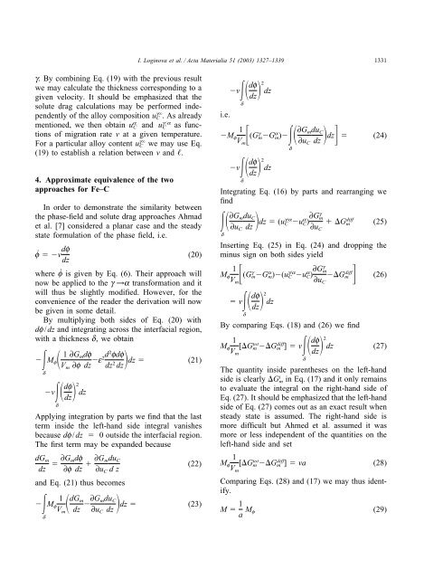
I. Loginova et al. / Acta Materialia 51 (2003) 1327–13391331g. By combining Eq. (19) with the previous resultwe may calculate the thickness corresponding to agiven velocity. It should be emphasized that thesolute drag calculations may be performed independentlyof the alloy composition uC g . As alreadymentioned, we then obtain u a C and uCg/a as functionsof migration rate v at a given temperature.For a particular alloy content u gC we may use Eq.(19) to establish a relation between v and .4. Approximate equivalence of the twoapproaches for Fe–CIn order to demonstrate the similarity betweenthe phase-field and solute drag approaches Ahmadet al. [7] considered a planar case and the steadystate formulation of the phase field, i.e.ḟ v df(20)dzwhere ḟ is given by Eq. (6). Their approach willnow be applied to the g →a transformation and itwill thus be slightly modified. However, for theconvenience of the reader the derivation will nowbe given in some detail.By multiplying both sides of Eq. (20) withdf/dz and integrating across the interfacial region,with a thickness d, we obtainM df 1∂G m df fdfV m ∂f dz e2d2 (21)dz dzdz 2v df 2dzdzdApplying integration by parts we find that the lastterm inside the left-hand side integral vanishesbecause df/dz 0 outside the interfacial region.The first term may be expanded becausedG mdz ∂G mdf∂f dz ∂G mdu C(22)∂u C dzand Eq. (21) thus becomes1M fVdm dG mdz ∂G mdu C∂u C dzdz (23)v df 2dzdzdi.e.1M fV m(G g mGm) ∂G a mdu C∂u C dzdz (24)dv df 2dzdzddIntegrating Eq. (16) by parts and rearranging wefind ∂G mdu C∂u C dzdz (u g/aC u a C) ∂Gg mG∂u diffm (25)CInserting Eq. (25) in Eq. (24) and dropping theminus sign on both sides yieldm (26)1M fVmGm(G g a m)(uC g/a u a C) ∂Gg m df dz vd2dz∂u CG diffBy comparing Eqs. (18) and (26) we find1M f [GV totm G diffm df 2dz (27)dzm ] vdThe quantity inside parentheses on the left-handside is clearly G i m in Eq. (17) and it only remainsto evaluate the integral on the right-hand side ofEq. (27). It should be emphasized that the left-handside of Eq. (27) comes out as an exact result whensteady state is assumed. The right-hand side ismore difficult but Ahmed et al. assumed it wasmore or less independent of the quantities on theleft-hand side and set1M f [GV totm G diffm ] va (28)mComparing Eqs. (28) and (17) we may thus identify.M 1 a M f (29)