- Page 1 and 2:
RePoSS: Research Publications on Sc
- Page 3 and 4:
The Mathematics of NIELS HENRIK ABE
- Page 5 and 6:
The Mathematics of NIELS HENRIK ABE
- Page 7 and 8:
Contents Contents i List of Tables
- Page 9 and 10:
8.3 Refocusing on the equation . .
- Page 11:
V ABEL’s mathematics and the rise
- Page 15 and 16:
List of Figures 2.1 NIELS HENRIK AB
- Page 17:
List of Boxes 1 The algebraic reduc
- Page 21 and 22:
Summary The present PhD dissertatio
- Page 23 and 24:
Preface to the 2004 edition For thi
- Page 25:
in connection with the Abel centenn
- Page 28 and 29:
items published in the same year ar
- Page 30 and 31:
the Mittag-Leffler archives in Djur
- Page 33 and 34:
Chapter 1 Introduction In the after
- Page 35 and 36:
1.2. The mathematical topics involv
- Page 37 and 38:
1.3. Themes from early nineteenth-c
- Page 39 and 40:
1.4. Reflections on methodology 9 l
- Page 41 and 42:
1.4. Reflections on methodology 11
- Page 43 and 44:
1.4. Reflections on methodology 13
- Page 45:
1.4. Reflections on methodology 15
- Page 48 and 49:
18 Chapter 2. Biography of NIELS HE
- Page 50 and 51:
20 Chapter 2. Biography of NIELS HE
- Page 52 and 53:
22 Chapter 2. Biography of NIELS HE
- Page 54 and 55:
24 Chapter 2. Biography of NIELS HE
- Page 56 and 57:
26 Chapter 2. Biography of NIELS HE
- Page 58 and 59:
28 Chapter 2. Biography of NIELS HE
- Page 60 and 61:
30 Chapter 2. Biography of NIELS HE
- Page 62 and 63:
32 Chapter 2. Biography of NIELS HE
- Page 64 and 65:
34 Chapter 2. Biography of NIELS HE
- Page 66 and 67:
36 Chapter 2. Biography of NIELS HE
- Page 69 and 70:
Chapter 3 Historical background The
- Page 71 and 72:
3.2. ABEL’s position in mathemati
- Page 73 and 74:
3.3. The state of mathematics 43 tr
- Page 75:
3.4. ABEL’s legacy 45 As can be s
- Page 79 and 80:
Chapter 4 The position and role of
- Page 81 and 82:
4.1. Outline of ABEL’s results an
- Page 83 and 84:
4.2. Mathematical change as a histo
- Page 85:
4.2. Mathematical change as a histo
- Page 88 and 89:
58 Chapter 5. Towards unsolvable eq
- Page 90 and 91:
60 Chapter 5. Towards unsolvable eq
- Page 92 and 93:
62 Chapter 5. Towards unsolvable eq
- Page 94 and 95:
64 Chapter 5. Towards unsolvable eq
- Page 96 and 97:
66 Chapter 5. Towards unsolvable eq
- Page 98 and 99:
68 Chapter 5. Towards unsolvable eq
- Page 100 and 101:
70 Chapter 5. Towards unsolvable eq
- Page 102 and 103:
72 Chapter 5. Towards unsolvable eq
- Page 104 and 105:
74 Chapter 5. Towards unsolvable eq
- Page 106 and 107:
76 Chapter 5. Towards unsolvable eq
- Page 108 and 109:
78 Chapter 5. Towards unsolvable eq
- Page 110 and 111:
80 Chapter 5. Towards unsolvable eq
- Page 112 and 113:
82 Chapter 5. Towards unsolvable eq
- Page 114 and 115:
84 Chapter 5. Towards unsolvable eq
- Page 116 and 117:
86 Chapter 5. Towards unsolvable eq
- Page 118 and 119:
88 Chapter 5. Towards unsolvable eq
- Page 120 and 121:
90 Chapter 5. Towards unsolvable eq
- Page 122 and 123:
92 Chapter 5. Towards unsolvable eq
- Page 124 and 125:
94 Chapter 5. Towards unsolvable eq
- Page 126 and 127:
96 Chapter 5. Towards unsolvable eq
- Page 128 and 129: 98 Chapter 6. Algebraic insolubilit
- Page 130 and 131: 100 Chapter 6. Algebraic insolubili
- Page 132 and 133: 102 Chapter 6. Algebraic insolubili
- Page 134 and 135: 104 Chapter 6. Algebraic insolubili
- Page 136 and 137: 106 Chapter 6. Algebraic insolubili
- Page 138 and 139: 108 Chapter 6. Algebraic insolubili
- Page 140 and 141: 110 Chapter 6. Algebraic insolubili
- Page 142 and 143: 112 Chapter 6. Algebraic insolubili
- Page 144 and 145: 114 Chapter 6. Algebraic insolubili
- Page 146 and 147: 116 Chapter 6. Algebraic insolubili
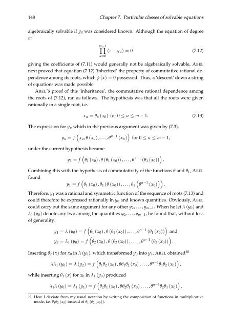
- Page 148 and 149: 118 Chapter 6. Algebraic insolubili
- Page 150 and 151: 120 Chapter 6. Algebraic insolubili
- Page 152 and 153: 122 Chapter 6. Algebraic insolubili
- Page 154 and 155: 124 Chapter 6. Algebraic insolubili
- Page 156 and 157: 126 Chapter 6. Algebraic insolubili
- Page 158 and 159: 128 Chapter 6. Algebraic insolubili
- Page 160 and 161: 130 Chapter 6. Algebraic insolubili
- Page 162 and 163: 132 Chapter 6. Algebraic insolubili
- Page 164 and 165: 134 Chapter 6. Algebraic insolubili
- Page 166 and 167: 136 Chapter 6. Algebraic insolubili
- Page 168 and 169: 138 Chapter 6. Algebraic insolubili
- Page 171 and 172: Chapter 7 Particular classes of equ
- Page 173 and 174: 7.1. Solubility of Abelian equation
- Page 175 and 176: 7.1. Solubility of Abelian equation
- Page 177: 7.1. Solubility of Abelian equation
- Page 181 and 182: 7.1. Solubility of Abelian equation
- Page 183 and 184: 7.2. Elliptic functions 153 Figure
- Page 185 and 186: 7.2. Elliptic functions 155 7.2.1 T
- Page 187 and 188: 7.3. The concept of irreducibility
- Page 189 and 190: 7.3. The concept of irreducibility
- Page 191: 7.4. Enlarging the class of solvabl
- Page 194 and 195: 164 Chapter 8. A grand theory in sp
- Page 196 and 197: 166 Chapter 8. A grand theory in sp
- Page 198 and 199: 168 Chapter 8. A grand theory in sp
- Page 200 and 201: 170 Chapter 8. A grand theory in sp
- Page 202 and 203: 172 Chapter 8. A grand theory in sp
- Page 204 and 205: 174 Chapter 8. A grand theory in sp
- Page 206 and 207: 176 Chapter 8. A grand theory in sp
- Page 208 and 209: 178 Chapter 8. A grand theory in sp
- Page 210 and 211: 180 Chapter 8. A grand theory in sp
- Page 212 and 213: 182 Chapter 8. A grand theory in sp
- Page 214 and 215: 184 Chapter 8. A grand theory in sp
- Page 216 and 217: 186 Chapter 8. A grand theory in sp
- Page 219: Part III Interlude: ABEL and the
- Page 222 and 223: 192 Chapter 9. The nineteenth-centu
- Page 224 and 225: 194 Chapter 10. Toward rigorization
- Page 226 and 227: 196 Chapter 10. Toward rigorization
- Page 228 and 229:
198 Chapter 10. Toward rigorization
- Page 230 and 231:
200 Chapter 10. Toward rigorization
- Page 232 and 233:
202 Chapter 10. Toward rigorization
- Page 234 and 235:
204 Chapter 10. Toward rigorization
- Page 236 and 237:
206 Chapter 10. Toward rigorization
- Page 238 and 239:
208 Chapter 11. CAUCHY’s new foun
- Page 240 and 241:
210 Chapter 11. CAUCHY’s new foun
- Page 242 and 243:
212 Chapter 11. CAUCHY’s new foun
- Page 244 and 245:
214 Chapter 11. CAUCHY’s new foun
- Page 246 and 247:
216 Chapter 11. CAUCHY’s new foun
- Page 248 and 249:
218 Chapter 11. CAUCHY’s new foun
- Page 251 and 252:
Chapter 12 ABEL’s reading of CAUC
- Page 253 and 254:
12.1. ABEL’s critical attitude 22
- Page 255 and 256:
12.1. ABEL’s critical attitude 22
- Page 257 and 258:
12.1. ABEL’s critical attitude 22
- Page 259 and 260:
12.3. Convergence 229 12.3 Converge
- Page 261 and 262:
12.3. Convergence 231 and {εm} was
- Page 263 and 264:
12.4. Continuity 233 it followed th
- Page 265 and 266:
12.4. Continuity 235 Actually, if t
- Page 267 and 268:
12.4. Continuity 237 DIRICHLET intr
- Page 269 and 270:
12.5. ABEL’s “exception” 239
- Page 271 and 272:
12.6. A curious reaction: Lehrsatz
- Page 273 and 274:
12.6. A curious reaction: Lehrsatz
- Page 275 and 276:
12.6. A curious reaction: Lehrsatz
- Page 277 and 278:
12.7. From power series to absolute
- Page 279 and 280:
12.7. From power series to absolute
- Page 281 and 282:
12.8. Product theorems of infinite
- Page 283 and 284:
12.8. Product theorems of infinite
- Page 285 and 286:
12.9. ABEL’s proof of the binomia
- Page 287 and 288:
12.9. ABEL’s proof of the binomia
- Page 289 and 290:
12.9. ABEL’s proof of the binomia
- Page 291 and 292:
12.10. Aspects of ABEL’s binomial
- Page 293:
12.10. Aspects of ABEL’s binomial
- Page 296 and 297:
266 Chapter 13. ABEL and OLIVIER on
- Page 298 and 299:
268 Chapter 13. ABEL and OLIVIER on
- Page 300 and 301:
270 Chapter 13. ABEL and OLIVIER on
- Page 302 and 303:
272 Chapter 13. ABEL and OLIVIER on
- Page 304 and 305:
274 Chapter 13. ABEL and OLIVIER on
- Page 307 and 308:
Chapter 14 Reception of ABEL’s co
- Page 309 and 310:
14.1. Reception of ABEL’s rigoriz
- Page 311 and 312:
14.2. Conclusion 281 of basic notio
- Page 313:
Part IV Elliptic functions and the
- Page 316 and 317:
286 Chapter 15. Elliptic integrals
- Page 318 and 319:
288 Chapter 15. Elliptic integrals
- Page 320 and 321:
290 Chapter 15. Elliptic integrals
- Page 322 and 323:
292 Chapter 15. Elliptic integrals
- Page 324 and 325:
294 Chapter 15. Elliptic integrals
- Page 326 and 327:
296 Chapter 15. Elliptic integrals
- Page 328 and 329:
298 Chapter 15. Elliptic integrals
- Page 330 and 331:
300 Chapter 16. The idea of inverti
- Page 332 and 333:
302 Chapter 16. The idea of inverti
- Page 334 and 335:
304 Chapter 16. The idea of inverti
- Page 336 and 337:
306 Chapter 16. The idea of inverti
- Page 338 and 339:
308 Chapter 16. The idea of inverti
- Page 340 and 341:
310 Chapter 16. The idea of inverti
- Page 342 and 343:
312 Chapter 16. The idea of inverti
- Page 344 and 345:
314 Chapter 16. The idea of inverti
- Page 346 and 347:
316 Chapter 16. The idea of inverti
- Page 348 and 349:
318 Chapter 16. The idea of inverti
- Page 351 and 352:
Chapter 17 Steps in the process of
- Page 353 and 354:
17.1. Infinite representations 323
- Page 355 and 356:
17.2. Elliptic functions as ratios
- Page 357 and 358:
17.2. Elliptic functions as ratios
- Page 359 and 360:
17.3. Characterization of ABEL’s
- Page 361 and 362:
Chapter 18 Tools in ABEL’s resear
- Page 363 and 364:
18.1. Transformation theory 333 The
- Page 365 and 366:
18.1. Transformation theory 335 Obv
- Page 367 and 368:
18.1. Transformation theory 337 Sum
- Page 369 and 370:
18.2. Integration in logarithmic te
- Page 371 and 372:
18.2. Integration in logarithmic te
- Page 373 and 374:
18.2. Integration in logarithmic te
- Page 375 and 376:
18.3. Conclusion 345 Summary. ABEL
- Page 377 and 378:
Chapter 19 The Paris memoir N. H. A
- Page 379 and 380:
19.1. ABEL’s approach to the Pari
- Page 381 and 382:
19.2. The contents of ABEL’s Pari
- Page 383 and 384:
19.2. The contents of ABEL’s Pari
- Page 385 and 386:
19.2. The contents of ABEL’s Pari
- Page 387 and 388:
19.2. The contents of ABEL’s Pari
- Page 389 and 390:
19.2. The contents of ABEL’s Pari
- Page 391 and 392:
19.2. The contents of ABEL’s Pari
- Page 393 and 394:
19.2. The contents of ABEL’s Pari
- Page 395 and 396:
19.2. The contents of ABEL’s Pari
- Page 397 and 398:
19.2. The contents of ABEL’s Pari
- Page 399 and 400:
19.2. The contents of ABEL’s Pari
- Page 401 and 402:
19.3. Additional, tentative remarks
- Page 403 and 404:
19.3. Additional, tentative remarks
- Page 405 and 406:
19.4. The fate of the Paris memoir
- Page 407 and 408:
19.6. Conclusion 377 hyperelliptic
- Page 409 and 410:
Chapter 20 General approaches to el
- Page 411 and 412:
20.2. Other ways of introducing ell
- Page 413:
20.3. Conclusion 383 All these four
- Page 417 and 418:
Chapter 21 ABEL’s mathematics and
- Page 419 and 420:
21.1. From formulae to concepts 389
- Page 421 and 422:
21.1. From formulae to concepts 391
- Page 423 and 424:
21.2. Concepts and classes enter ma
- Page 425 and 426:
21.3. The role of counter examples
- Page 427 and 428:
21.3. The role of counter examples
- Page 429 and 430:
21.3. The role of counter examples
- Page 431:
21.4. Conclusion 401 It is beyond t
- Page 434 and 435:
404 Appendix A. ABEL’s correspond
- Page 437 and 438:
Appendix B ABEL’s manuscripts Man
- Page 439 and 440:
1. Précis d’une théorie des fon
- Page 441 and 442:
Bibliography Abel (MS:351:A). “M
- Page 443 and 444:
Bibliography 413 in: Journal für d
- Page 445 and 446:
Bibliography 415 — (1990). “Geo
- Page 447 and 448:
Bibliography 417 — (1830). “Mé
- Page 449 and 450:
Bibliography 419 — (1768). “Ins
- Page 451 and 452:
Bibliography 421 Grattan-Guinness,
- Page 453 and 454:
Bibliography 423 Jahnke, H. N. (198
- Page 455 and 456:
Bibliography 425 Legendre, A. M. (1
- Page 457 and 458:
Bibliography 427 Rosen, M. (1981).
- Page 459:
Bibliography 429 Toti Rigatelli, L.
- Page 462 and 463:
432 Index of names Frobenius, Georg
- Page 465 and 466:
Index École Normale, 40, 187 Écol
- Page 467:
Index 437 Lagrange interpolation, 3
- Page 470:
RePoSS (Research Publications on Sc