Diez lecciones sobre Sistemas Hamiltonianos, Integrabilidad y ...

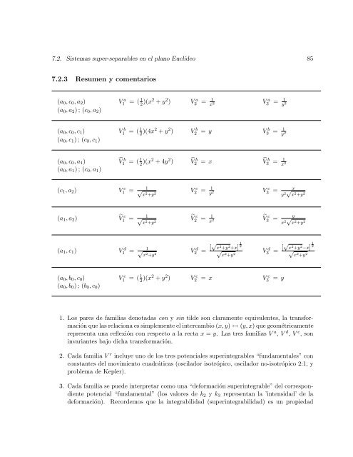
7.2. Sistemas super-separables en el plano Euclídeo 85
7.2.3 Resumen y comentarios
(a0, c0, a2) V a
1
(a0, a2) ; (c0, a2)
(a0, c0, c1) V b
1
(a0, c1) ; (c0, c1)
(a0, c0, a1)
(a0, a1) ; (c0, a1)
1 = ( 2 )(x2 + y2 ) V a
2
1 = ( 2 )(4x2 + y2 ) V b
2
V b
1 = ( 1
2 )(x2 + 4y 2 )
(c1, a2) V c
1 = √ 1
x2 +y2 (a1, a2)
V c 1
1 = √
x2 +y2 (a1, c1) V d
1 = √ 1
x2 +y2 (a0, b0, c0) V e
1
(a0, b0) ; (b0, c0)
= 1
x 2
V a
3
= y V b
3
= 1
y 2
= 1
y 2
V b
2 = x V b
3 = 1
x 2
V c
2
V c
2
1 = ( 2 )(x2 + y2 ) V e
2
= 1
y 2
= 1
x 2
V d
2 = [√x2 +y2 +x] 1 2
√
x2 +y2 = x V e
3
V c
3 = x
y 2√ x 2 +y 2
V c
3 =
y
x 2√ x 2 +y 2
V d
3 = [√x2 +y2−x] 1 2
√
x2 +y2 1. Los pares de familias denotadas con y sin tilde son claramente equivalentes, la transformación
que las relaciona es simplemente el intercambio (x, y) ↔ (y, x) que geométricamente
representa una reflexión con respecto a la recta x = y. Las tres familias V a , V d , V e , son
invariantes bajo dicha transformación.
2. Cada familia V r incluye uno de los tres potenciales superintegrables “fundamentales” con
constantes del movimiento cuadráticas (oscilador isotrópico, oscilador no-isotrópico 2:1, y
problema de Kepler).
3. Cada familia se puede interpretar como una “deformación superintegrable” del correspondiente
potencial “fundamental” (los valores de k2 y k3 representan la ’intensidad’ de la
deformación). Recordemos que la integrabilidad (superintegrabilidad) es un propiedad
= y