- Page 1 and 2:
BUDAPESTI CORVINUS EGYETEM A VÁLLA
- Page 3 and 4:
PÉNZÜGYI ÉS SZÁMVITELI INTÉZET
- Page 6 and 7:
TARTALOMJEGYZÉK TARTALOMJEGYZÉK..
- Page 8 and 9:
VI.2. AZ ELEMZÉS KÉRDÉSFELTEVÉS
- Page 10 and 11:
A.15 - 9. táblázat ..............
- Page 12 and 13:
33. B ábra - Az eredeti és hedgel
- Page 14 and 15:
kockázatokban rejlő lehetőségek
- Page 16 and 17:
szerkezeti, növekedési és kocká
- Page 18 and 19:
Hatás a belső allokálásra A vá
- Page 20 and 21:
aktív trading révén arbitrázs n
- Page 22 and 23:
feltétel teljesíthető, amennyibe
- Page 24 and 25:
eredetileg angol nyelven írtam, az
- Page 26 and 27:
vállalatéval azonos feltételek m
- Page 28 and 29:
veszteség jelentőségét, s kés
- Page 30 and 31:
Újfent fontos felismernünk azt, h
- Page 32 and 33:
finanszírozási tevékenységekkel
- Page 34 and 35:
Legtöbbször azonban sem a megbíz
- Page 36 and 37:
meghatározott cégértékre felír
- Page 38 and 39:
Kockázatnövelés és a követelé
- Page 40 and 41:
definiálják azokat a körülmény
- Page 42 and 43:
eszközök, feltéve, hogy a kezele
- Page 44 and 45:
felár meghatározásakor a fedezé
- Page 46 and 47:
ámutatnak arra is, hogy a rövid l
- Page 48 and 49:
hogy hasznossági függvénye a cé
- Page 50 and 51:
izonyul, mivel a cégvezetés szám
- Page 52 and 53:
megváltoztatni úgy, hogy felfedje
- Page 54 and 55:
kockázatkezelés tekintetében. Mi
- Page 56 and 57:
Breeden és Viswanathan [1998] ered
- Page 58 and 59:
a vállalat kitettségeinek nyilvá
- Page 60 and 61:
jelenti az egyensúlyi fedezési po
- Page 62 and 63:
előnyben részesítik az új rész
- Page 64 and 65:
Mint Froot et al. [1993] rámutat,
- Page 66 and 67:
ákényszerítése arra, hogy beruh
- Page 68 and 69:
stratégiák haszna kisebb, mivel a
- Page 70 and 71:
A Froot-Schaferstein-Stein [1993] m
- Page 72 and 73:
termékárakra azt eredményezi, ho
- Page 74 and 75:
viszonylag állandó ágazati árak
- Page 76 and 77:
erősségére, ezáltal pedig strat
- Page 78 and 79:
III. 2. A kockázat-tudatos vállal
- Page 80 and 81:
III. 2. 1. A stratégiai kockázato
- Page 82 and 83:
pénzügyi eszközök piacára jell
- Page 84 and 85:
A gazdasági tőkén alapuló vezet
- Page 86 and 87:
pontosabb teljesítményértékelé
- Page 88 and 89:
(üzleti területek, projektek) kö
- Page 90 and 91:
IV. A VÁLLALATI KOCKÁZATKEZELÉS
- Page 92 and 93:
IV. 2. A vállalati szintű kockáz
- Page 94 and 95:
csökkentése mellett (hitelkovená
- Page 96 and 97:
azok a kovenánsok, amelyek visszat
- Page 98 and 99:
V. SZINOPSZIS A RÉSZVÉNYESI ÉRT
- Page 100 and 101:
(túlmutatva a hagyományos vállal
- Page 102 and 103:
kockázatkezelési politika megvál
- Page 104 and 105:
torzításhoz vezethet bármilyen,
- Page 106 and 107:
Leland [1994] a vállalat piaci ér
- Page 108 and 109:
elérhető értéktöbbletet száms
- Page 110 and 111:
továbbiakban, s ezért az eszközh
- Page 112 and 113:
VI.3. A vállalati értékfolyamat
- Page 114 and 115:
A vállalat egy m. periódusban gen
- Page 116 and 117:
[ F ] μ [ F { P + Δ }] − [ F {
- Page 118 and 119:
[23. és 24. ábrák] VI.4. Az ipar
- Page 120 and 121:
Hipotézis 3 Amennyiben a piacon n=
- Page 122 and 123:
Z = n n, k 1 m n ∑ j= 1 S [ m+ n
- Page 124 and 125:
Var n, i [ Z ] 0 Var 0 m [ P ] m n
- Page 126 and 127:
kombinációjának szórása az egy
- Page 128 and 129:
[ H ] μ [ H { P + Δ }] − [ H {
- Page 130 and 131:
Az első típusú hatás csak addig
- Page 132 and 133:
Fontos látni azt is, hogy egyperi
- Page 134 and 135:
(azaz a tőkeáttétel százazalék
- Page 136 and 137:
AVA'' 1+ PB IC D'' E = − = AVA' 1
- Page 138 and 139: arányosan nő a tranzakciós költ
- Page 140 and 141: VII. A FINOMíTÓ IPARBAN ELÉRHET
- Page 142 and 143: 2. lépés - lineáris függőség
- Page 144 and 145: szórással. A 44. ábráról is j
- Page 146 and 147: A vállalatokra 1990-től sikerült
- Page 148 and 149: normál érték háromszorosa eset
- Page 150 and 151: IRODALOMJEGYZÉK Acharya, V., and C
- Page 152 and 153: Bodnar, G. M., Hayt, G. S., and Mar
- Page 154 and 155: Dunis, C. L., Laws, J., and Evans,
- Page 156 and 157: Hill, C., and Snell, S., [1988], Ex
- Page 158 and 159: Lintner, J., [1965], The Valuation
- Page 160 and 161: Sharpe, W. F., [1964], Capital Asse
- Page 162 and 163: FÜGGELÉKEK 161
- Page 164 and 165: 2. függelék - Likviditáskockáza
- Page 166 and 167: in terms of expected utility. There
- Page 168 and 169: His comparative statics results sug
- Page 170 and 171: 4. függelék - A Smith-Stulz [1985
- Page 172 and 173: 5. függelék - A vezetői kompenz
- Page 174 and 175: 6. függelék - A Guay-Haushalter-M
- Page 176 and 177: 7. függelék - Az FSS modell levez
- Page 178 and 179: Adam [2002] gives empirical support
- Page 180 and 181: 9. függelék - Az FSS [1993] féle
- Page 182 and 183: Adam et al. [2004] show that an int
- Page 184 and 185: This term is assumed to be increasi
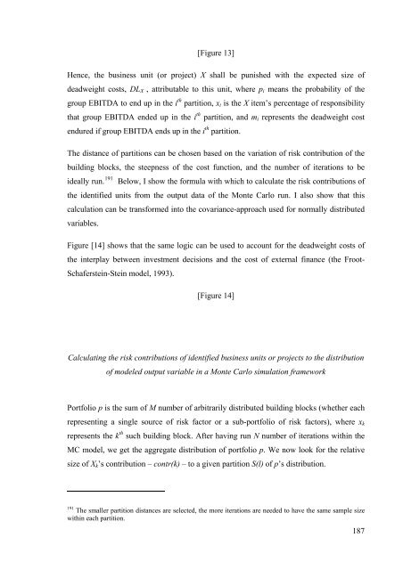
- Page 186 and 187: situations of both firms, with the
- Page 190 and 191: Contr (k) = N ∑ ⎡ ⎢ ⎣ M k k
- Page 192 and 193: increases. Their results suggest th
- Page 194 and 195: A Haushalter-Heron-Lie [2002] model
- Page 196 and 197: Lookman [2005b] conducts the analys
- Page 198 and 199: managers might hedge to ensure suff
- Page 200 and 201: derivatives purely for hedging, the
- Page 202 and 203: The firm defaults when asset value
- Page 204 and 205: In a second stage optimization, Lel
- Page 206 and 207: even if the distance-to-default - m
- Page 208 and 209: dolgoztam. Továbbá mellőzöm az
- Page 210 and 211: faktorok vonatkozásában alkalmaza
- Page 212 and 213: főkomponens elemzésre, 0.5-0.7 k
- Page 214 and 215: A kapott 6 db főkomponenssel, mint
- Page 216 and 217: standardizált értékeiből állna
- Page 218 and 219: TÁBLÁZATOK 217
- Page 220 and 221: 3. táblázat - A kockázatkezelés
- Page 222 and 223: A.15 - 2. táblázat Model Summary
- Page 224 and 225: A.15 - 5. táblázat Communalities
- Page 226 and 227: A.15 - 9. táblázat BRENT PUN_CR E
- Page 228 and 229: A.15 - 13. táblázat Collinearity
- Page 230 and 231: A.15 - 15. táblázat és grafikono
- Page 232 and 233: A.15 - 18. táblázat 1000 tonna F0
- Page 234 and 235: 1. ábra - Értékteremtés kockáz
- Page 236 and 237: 4. ábra - Az adózás után válla
- Page 238 and 239:
7. ábra - Elkülönülő és köz
- Page 240 and 241:
9. ábra - Az optimális fedezeti r
- Page 242 and 243:
12. ábra - Kockázati hozzájárul
- Page 244 and 245:
15. ábra - A fedezés hatása a Ro
- Page 246 and 247:
16. B ábra - A vállalati kockáza
- Page 248 and 249:
17. B ábra - Eszközhozam lehetsé
- Page 250 and 251:
19. ábra - Az eszközhozam folyama
- Page 252 and 253:
23. ábra - Az iparági eszközhoza
- Page 254 and 255:
25. B ábra - Az eszközhozam folya
- Page 256 and 257:
28. ábra- Eltérő futamidejű swa
- Page 258 and 259:
30. ábra - Az eltérő gyakoriság
- Page 260 and 261:
32. ábra - A hedgelt vállalati PB
- Page 262 and 263:
33. B ábra - Az eredeti és hedgel
- Page 264 and 265:
35. ábra - Eltérő futamidejű sw
- Page 266 and 267:
38. ábra - A részvényesi PB vál
- Page 268 and 269:
41. ábra - A részvényesi PB vál
- Page 270 and 271:
43. ábra - Az USGC dízelolaj és
- Page 272 and 273:
47. ábra - A kiinduló dízelolaj