fundamentals of engineering supplied-reference handbook - Ventech!

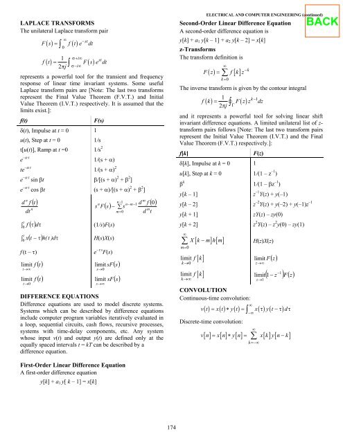
LAPLACE TRANSFORMS
The unilateral Laplace transform pair
∞ −st
0
( ) = ∫ ( )
F s f t e dt
1 σ+ i∞ st
f () t = F( s) e dt
2πj
∫ σ−i∞ represents a powerful tool for the transient and frequency
response of linear time invariant systems. Some useful
Laplace transform pairs are [Note: The last two transforms
represent the Final Value Theorem (F.V.T.) and Initial
Value Theorem (I.V.T.) respectively. It is assumed that the
limits exist.]:
f(t) F(s)
δ(t), Impulse at t = 0 1
u(t), Step at t = 0 1/s
t[u(t)], Ramp at t =0 1/s 2
–α t
e
1/(s + α)
te –α t 1/(s + α) 2
e –α t sin βt β/[(s + α) 2 + β 2 ]
e –α t cos βt (s + α)/[(s + α) 2 + β 2 ]
n
d f
dt
t
() t
n
() τ
s
n
F
() s
∫0
f dτ
(1/s)F(s)
∫
( t − τ)
t
0 x h(
t ) dτ
H(s)X(s)
f (t – τ) e –τ s F(s)
limit f () t
limit sF()
s
t→∞ limit
t→0 f () t
s→0 limit
s→∞ n 1
n m 1
− ∑ s
m 0
−
− −
=
sF()
s
m
d f
m
d t
( 0)
DIFFERENCE EQUATIONS
Difference equations are used to model discrete systems.
Systems which can be described by difference equations
include computer program variables iteratively evaluated in
a loop, sequential circuits, cash flows, recursive processes,
systems with time-delay components, etc. Any system
whose input v(t) and output y(t) are defined only at the
equally spaced intervals t = kT can be described by a
difference equation.
First-Order Linear Difference Equation
A first-order difference equation
y[k] + a1 y[ k – 1] = x[k]
174
ELECTRICAL AND COMPUTER ENGINEERING (continued)
Second-Order Linear Difference Equation
A second-order difference equation is
y[k] + a1 y[k – 1] + a2 y[k – 2] = x[k]
z-Transforms
The transform definition is
∞
F( z) = ∑ f [ k] z
k=
0
−k
The inverse transform is given by the contour integral
1
k −1
f ( k) = F( z) z dz
2πj
∫� Γ
and it represents a powerful tool for solving linear shift
invariant difference equations. A limited unilateral list of ztransform
pairs follows [Note: The last two transform pairs
represent the Initial Value Theorem (I.V.T.) and the Final
Value Theorem (F.V.T.) respectively.]:
f[k] F(z)
δ[k], Impulse at k = 0 1
u[k], Step at k = 0 1/(1 – z –1 )
β k
1/(1 – βz –1 )
y[k – 1]
z –1 Y(z) + y(–1)
y[k – 2] z –2 Y(z) + y(–2) + y(–1)z –1
y[k + 1] zY(z) – zy(0)
y[k + 2] z 2 Y(z) – z 2 y(0) – zy(1)
∞
∑ X [ k − m] h[ m]
H(z)X(z)
m=
0
k→0
[ ]
limit f k
[ ]
limit f k
k→∞
CONVOLUTION
Continuous-time convolution:
limit F
z→∞ limit
z→1
( z)
−1
( 1−
z ) F(
z)
() () () ∫ ( ) ( )
vt = xt∗ yt = xτ yt−τ dτ
Discrete-time convolution:
∞
−∞
[ ] = [ ] ∗ [ ] = ∑
[ ] [ − ]
vn xn yn xk yn k
∞
k =−∞