fundamentals of engineering supplied-reference handbook - Ventech!

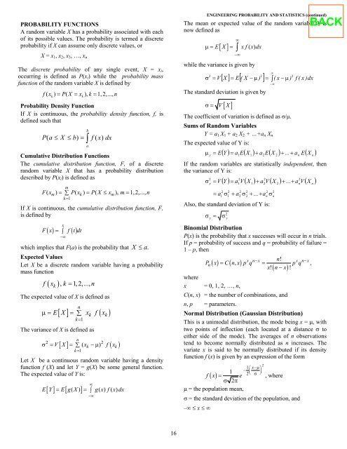
PROBABILITY FUNCTIONS
A random variable X has a probability associated with each
of its possible values. The probability is termed a discrete
probability if X can assume only discrete values, or
X = x1, x2, x3, …, xn
The discrete probability of any single event, X = xi,
occurring is defined as P(xi) while the probability mass
function of the random variable X is defined by
f k
k
( x ) = P(
X = x ), k = 1, 2, ..., n
Probability Density Function
If X is continuous, the probability density function, f, is
defined such that
P ( a ≤ X ≤ b)
= f ( x)
dx
b
∫
a
Cumulative Distribution Functions
The cumulative distribution function, F, of a discrete
random variable X that has a probability distribution
described by P(xi) is defined as
m
m
∑
k=
1
k m
F( x ) = P( x ) = P( X ≤ x ), m= 1,2,..., n
If X is continuous, the cumulative distribution function, F,
is defined by
x
( ) = ∫ ( )
F x f t dt
−∞
which implies that F(a) is the probability that X ≤ a.
Expected Values
Let X be a discrete random variable having a probability
mass function
f ( x ), k = 1,2,..., n
k
The expected value of X is defined as
n
[ ] ( )
µ= E X = ∑ x f x
k=
1
The variance of X is defined as
k k
n
2 2
V X xk f xk
k=
1
[ ] ∑ ( ) ( )
σ = = −µ
Let X be a continuous random variable having a density
function f (X) and let Y = g(X) be some general function.
The expected value of Y is:
[ ] [ ]
E Y = E g( X) = ∫ g( x) f( x) dx
∞
−∞
16
ENGINEERING PROBABILITY AND STATISTICS (continued)
The mean or expected value of the random variable X is
now defined as
∞
µ= E[ X] = ∫ xf( x) dx
−∞
while the variance is given by
∞
2
[ X ] = E[
( X − µ ) ] = ∫
2
2
σ = V
( x − µ ) f ( x ) dx
The standard deviation is given by
σ=
V[ X]
−∞
The coefficient of variation is defined as σ/µ.
Sums of Random Variables
Y = a1 X1 + a2 X2 + …+an Xn
The expected value of Y is:
( Y ) = a E(
X ) + a E(
X ) + ... a E(
X )
µ y =
1 1 2 2
E +
If the random variables are statistically independent, then
the variance of Y is:
σ
2
y
= V
2
2
2
( Y ) = a V ( X ) + a V ( X ) + ... + a V ( X )
1
= a σ + a σ + ... + a σ
2 2 2 2
2 2
1 1 2 2
n n
Also, the standard deviation of Y is:
σ
y
=
σ
2
y
1
Binomial Distribution
P(x) is the probability that x successes will occur in n trials.
If p = probability of success and q = probability of failure =
1 – p, then
x n−x n!
x n−x Pn ( x) = Cnxpq ( , ) = pq ,
x! ( n−x) !
where
x = 0, 1, 2, …, n,
C(n, x) = the number of combinations, and
n, p = parameters.
Normal Distribution (Gaussian Distribution)
This is a unimodal distribution, the mode being x = µ, with
two points of inflection (each located at a distance σ to
either side of the mode). The averages of n observations
tend to become normally distributed as n increases. The
variate x is said to be normally distributed if its density
function f (x) is given by an expression of the form
1
f ( x) = e
σ 2π
µ = the population mean,
2
2
1⎛
x−µ
⎞
− ⎜ ⎟
2⎝
σ ⎠
2
, where
σ = the standard deviation of the population, and
–∞ ≤ x ≤ ∞
n
n
n
n