fundamentals of engineering supplied-reference handbook - Ventech!

Signal Conditioning
Signal conditioning of the measured analog signal is often
required to prevent alias frequencies and to reduce
measurement errors. For information on these signal
conditioning circuits, also known as filters, see the
ELECTRICAL AND COMPUTER ENGINEERING
section.
MEASUREMENT UNCERTAINTY
Suppose that a calculated result R depends on measurements
whose values are x1 ± w1, x2 ± w2, x3 ± w3, etc., where R =
f(x1, x2, x3, … xn), xi is the measured value, and wi is the
uncertainty in that value. The uncertainty in R, wR, can be
estimated using the Kline-McClintock equation:
2
2
2
1 2
⎟
1
2
⎟
∂f
⎞ ⎛ ∂f
⎞ ⎛ ∂f
⎞
⎟ +
⎜ w
⎟ + + ⎜
∂ ∂ ⎜
wn
x x
∂xn
⎛
wR =
⎜ w
…
⎝ ⎠ ⎝ ⎠
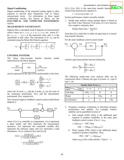
CONTROL SYSTEMS
The linear time-invariant transfer function model
represented by the block diagram
X(s)
can be expressed as the ratio of two polynomials in the form
Y
X
() s
() s
() s
() s
M
∏
N
= G()
s = = K N
D
m=
1
∏
n=
1
⎝
( s − z )
m
( s − p )
where the M zeros, zm, and the N poles, pn, are the roots of
the numerator polynomial, N(s), and the denominator
polynomial, D(s), respectively.
One classical negative feedback control system model block
diagram is
where G1(s) is a controller or compensator, G2(s) represents
a plant model, and H(s) represents the measurement
dynamics. Y(s) represents the controlled variable, R(s)
represents the reference input, and L(s) represents a load
disturbance. Y(s) is related to R(s) and L(s) by
G1
()
() s G2()
s
Y s =
R()
s
1+
G s G s H s
1
+
1+
G(s)
() 2()
()
G2()
s
G () s G () s H () s
1
2
Y(s)
L
() s
n
⎠
Y
88
MEASUREMENT AND CONTROLS (continued)
G1(s) G2(s) H(s) is the open-loop transfer function. The
closed-loop characteristic equation is
1 + G1(s) G2(s) H(s) = 0
System performance studies normally include:
1. Steady-state analysis using constant inputs is based on
the Final Value Theorem. If all poles of a G(s) function
have negative real parts, then
Steady State Gain = limG() s
s→0
Note that G(s) could refer to either an open-loop or a closedloop
transfer function.
For the unity feedback control system model
with the open-loop transfer function defined by
G
() s
K
=
s
B
T
M
( 1+
s )
∏ ω
m=
1 × N
∏ ω
n=
1
m
( 1+
s )
The following steady-state error analysis table can be
constructed where T denotes the type of system; i.e., type 0,
type 1, etc.
Steady-State Error ess
Input Type T = 0 T = 1 T = 2
Unit Step 1/(KB + 1) 0 0
Ramp ∞ 1/KB 0
Acceleration ∞ ∞ 1/KB
2. Frequency response evaluations to determine dynamic
performance and stability. For example, relative
stability can be quantified in terms of
a. Gain margin (GM) which is the additional gain
required to produce instability in the unity gain
feedback control system. If at ω = ω180,
∠ G(jω180) = –180°; then
GM = –20log10 (⏐G(jω180)⏐)
b. Phase margin (PM) which is the additional phase
required to produce instability. Thus,
PM = 180° + ∠ G(jω0dB)
where ω0dB is the ω that satisfies ⏐G(jω)⏐ = 1.
n
Y