fundamentals of engineering supplied-reference handbook - Ventech!

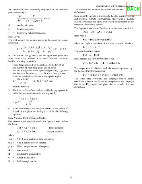
An alternative form commonly employed in the chemical
process industry is
Y() s K
= , where
Rs () 2 2
τ s + 2ζτ s+
1
K = steady state gain,
ζ = the damping ratio,
τ = the inverse natural frequency.
Root Locus
The root locus is the locus of points in the complex s-plane
satisfying
( s−z1)( s−z2) �(
s−zm) 1+ K = 0 m≤n ( s− p1)( s− p2) �(
s− pn)
as K is varied. The pi and zj are the open-loop poles and
zeros, respectively. When K is increased from zero the locus
has the following properties.
1. Locus branches exist on the real axis to the left of an
odd number of open-loop poles and/or zeros
2. The locus originates at the open-loop poles p1,…, pn and
terminates at the zeros z1,…, zm. If m < n then (n – m)
branches terminate at infinity at asymptote angles
(2k + 1)180°
α= k = 0, ± 1, ± 2, ± 3, �
n−m with the real axis.
3. The intersection of the real axis with the asymptotes is
called the asymptote centroid and is given by
σ =
A
n m
∑ pi − ∑ zi
i= 1 i=
1
Re( ) Re( )
n−m 4. If the locus crosses the imaginary (ω) axis the values of
K and ω are given by letting s = jω in the defining
equation.
State-Variable Control-System Models
One common state-variable model for dynamic systems has
the form
x�
(t) = Ax(t) + Bu(t) (state equation)
y(t) = Cx(t) + Du(t) (output equation)
where
x(t)
= N by 1 state vector (N state variables),
u(t) = R by 1 input vector (R inputs),
y(t) = M by 1 output vector (M outputs),
A = system matrix,
B = input distribution matrix,
C = output matrix, and
D = feed-through matrix.
90
MEASUREMENT AND CONTROLS (continued)
The orders of the matrices are defined via variable
definitions.
State-variable models automatically handle multiple inputs
and multiple outputs. Furthermore, state-variable models
can be formulated for open-loop system components or the
complete closed-loop system.
The Laplace transform of the time-invariant state equation is
sX(s) – x(0) = AX(s) + BU(s)
from which
X(s) = Φ(s) x(0) + Φ(s) BU(s)
where the Laplace transform of the state transition matrix is
Φ(s) = [sI – A] –1 .
The state-transition matrix
Φ(t) = L –1 {Φ(s)}
(also defined as e At ) can be used to write
x(t) = Φ(t) x(0) + ∫ t
Φ (t – τ) Bu(τ) dτ
0
The output can be obtained with the output equation; e.g.,
the Laplace transform output is
Y(s) = {CΦ(s) B + D}U(s) + CΦ(s) x(0)
The latter term represents the output(s) due to initial
conditions whereas the former term represents the output(s)
due to the U(s) inputs and gives rise to transfer function
definitions.