fundamentals of engineering supplied-reference handbook - Ventech!

Poisson Input—Arbitrary Service Time
Variance σ 2 is known. For constant service time,
σ 2 = 0.
P0 = 1 – ρ
Lq = (λ 2 σ 2 + ρ 2 )/[2 (1 – ρ)]
L = ρ + Lq
Wq = Lq / λ
W = Wq + 1/µ
Poisson Input—Erlang Service Times, σ 2 = 1/(kµ 2 )
Lq = [(1 + k)/(2k)][(λ 2 )/(µ (µ– λ))]
= [λ 2 /(kµ 2 ) + ρ 2 ]/[2(1 – ρ)]
Wq = [(1 + k)/(2k)]{λ /[µ (µ – λ)]}
W = Wq + 1/µ
Multiple Server Model (s > 1)
Poisson Input—Exponential Service Times
⎡ n s
⎛λ⎞ ⎛λ⎞ ⎤
⎢
⎛ ⎞
s−1
⎜ ⎟ ⎜ ⎟ ⎥
⎢ ⎝µ⎠ ⎝µ⎠ ⎜ 1 ⎟⎥
P0
= ⎢∑+ ⎜ ⎟
n=
0 n! s!
λ ⎥
⎢ ⎜1−⎟⎥ ⎢ ⎝ sµ⎠
⎣
⎥
⎦
L
q
s−1
n s
( sρ) ( sρ)
∑ n! s!1
( −ρ)
⎡ ⎤
= 1 ⎢ + ⎥
⎢ ⎥
⎣n= 0
⎦
⎛λ⎞ P0
⎜
⎝µ⎠
⎟
=
s!1
Ps
=
s!1
s
( −ρ)
( −ρ)
ρ
2
s s+
1
0 ρ
2
Pn = P0 (λ/µ) n /n! 0 ≤ n ≤ s
Pn = P0 (λ/µ) n /(s! s n – s ) n ≥ s
Wq = Lq/λ
W = Wq + 1/µ
L = Lq + λ/µ
Calculations for P0 and Lq can be time consuming; however,
the following table gives formulas for 1, 2, and 3 servers.
−1
s P0 Lq
1 1 – ρ ρ 2 /(1 – ρ)
2 (1 – ρ)/(1 + ρ) 2ρ 3 /(1 – ρ 2 )
3 2(
1−
ρ)
2
2 + 4ρ
+ 3ρ
4
9ρ
2 3
2 + 2ρ
− ρ − 3ρ
191
INDUSTRIAL ENGINEERING (continued)
SIMULATION
1. Random Variate Generation
The linear congruential method of generating pseudorandom
numbers Ui between 0 and 1 is obtained using
Zn = (aZn+C) (mod m) where a, C, m, and Zo are given nonnegative
integers and where Ui = Zi /m. Two integers are
equal (mod m) if their remainders are the same when
divided by m.
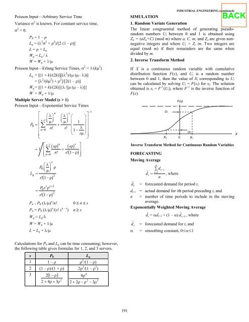
2. Inverse Transform Method
If X is a continuous random variable with cumulative
distribution function F(x), and Ui is a random number
between 0 and 1, then the value of Xi corresponding to Ui
can be calculated by solving Ui = F(xi) for xi. The solution
obtained is xi = F –1 (Ui), where F –1 is the inverse function of
F(x).
U1 U1
F(x)
1
U2
U2
X2 X1
X2
Inverse Transform Method for Continuous Random Variables
FORECASTING
Moving Average
n
X2 0
d
d
n
ˆ
∑ t i
i
t = =
−
1 , where
d ˆ
t = forecasted demand for period t,
dt–i = actual demand for ith period preceding t, and
n = number of time periods to include in the moving
average.
Exponentially Weighted Moving Average
dt ˆ = αdt–1 + (1 – α) dt 1
ˆ , where
dt ˆ = forecasted demand for t, and
α = smoothing constant, 0≤α≤1
−
X X