On the Flavor Problem in Strongly Coupled Theories - THEP Mainz

More documents

Recommendations

Info

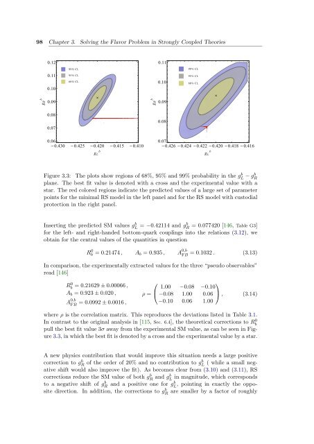
98 Chapter 3. Solving the Flavor Problem in Strongly Coupled Theories gR b 0.12 0.11 0.10 0.09 0.08 0.07 99� CL 95� CL 68� CL � 0.06 �0.430 �0.425 �0.420 �0.415 �0.410 � gL b gR b 0.11 0.10 0.09 0.08 99� CL 95� CL 68� CL 0.07 �0.426 �0.424 �0.422 �0.420 �0.418 �0.416 Figure 3.3: The plots show regions of 68%, 95% and 99% probability in the g b L − gb R plane. The best fit value is denoted with a cross and the experimental value with a star. The red colored regions indicate the predicted values of a large set of parameter points for the minimal RS model in the left panel and for the RS model with custodial protection in the right panel. Inserting the predicted SM values gb L = −0.42114 and gb R = 0.077420 [146, Table G3] for the left- and right-handed bottom-quark couplings into the relations (3.12), we obtain for the central values of the quantities in question R 0 b = 0.21474 , Ab = 0.935 , A 0,b FB = 0.1032 . (3.13) In comparison, the experimentally extracted values for the three “pseudo observables” read [146] R0 b = 0.21629 ± 0.00066 , Ab = 0.923 ± 0.020 , A 0,b FB = 0.0992 ± 0.0016 , � gL b ⎛ 1.00 −0.08 ⎞ −0.10 ρ = ⎝ −0.08 1.00 0.06 ⎠ , (3.14) −0.10 0.06 1.00 where ρ is the correlation matrix. This reproduces the deviations listed in Table 3.1. In contrast to the original analysis in [115, Sec. 6.4], the theoretical corrections to R 0 b pull the best fit value 3σ away from the experimental SM value, as can be seen in Figure 3.3, in which the best fit is denoted by a cross and the experimental value by a star. A new physics contribution that would improve this situation needs a large positive correction to gb R of the order of 20% and no contribution to gb L ( while a small negative shift would also improve the fit). As becomes clear from (3.10) and (3.11), RS corrections reduce the SM value of both gb R and gb L in magnitude, which corresponds to a negative shift of gb R and a positive one for gb L , pointing in exactly the oppo- are smaller by a factor of roughly site direction. In addition, the corrections to g b R �
δg b R /δgb L ∼ F (cbR )2 /F (cbL )2 for δg b = (g b RS −gb SM )/gb SM 3.1. Electroweak Precision Observables 99 , which is typically of the order of a few percent, because cbL is more IR localized in order to help realizing the large top mass in (2.158). The scaling on the plot in the left panel of Figure 3.3 however makes the gb R corrections completely invisible. As a consequence, our set of parameter points, which is chosen so that the correct quark masses and mixings are reproduced (see Appendix A for details), lies entirely in the red band shown in the left panel of Figure 3.3 and therefore fails to agree with the experiment within 3σ for the majority of points. Note, that the scaling of Figure 3.3 distorts the fact that there are still 10% of the parameter points in the 3σ ellipse. Translating this into a constraint for MKK would yield a very strong bound. One can invoke the reparametrization invariance introduced in section 2.5 in order to examine the characteristics of the parameter corner which is in agreement with this constraint. By reshuffling between F (cbL ) and F (cbR ) using (2.169), for η < 1, one increases δgb R /δgb L . For η = 1/2(1/3), about 35(45)% of the parameter points do at least not aggravate the already large discrepancy between the SM and the experiment. Thus, parameter points with strongly IR localized right-handed bottom quarks tend to give less dangerous corrections to the global fit in (3.14). It is interesting to discuss the implications for the dual theory of such a considerable reparametrization. Scaling down F (cbL ) will not only enlarge F (cbR ), but also F (ctR ), the zero mode of the right-handed top, which is already strongly IR localized. In a generalization of this shift to all generations, one can assume that all doublets are extremely UV localized and all singlets shifted towards the IR. The dual theory of such a model would have, to a good approximation, only right-handed quarks composites, while the left-handed quarks are elementaries. This right-handed compositeness was found to be a very attractive idea in [149], in which the relevance for the Z¯bb vertex was however not pointed out. In the later sections we will get back to this scenario and check the compatibility with other observables. This situation is also ameliorated by the mixing between the Z zero mode and the additional neutral composite vector bosons of the SU(2)R present in the custodially protected RS model [148]. This is especially intriguing, because as discussed in the previous section, the scalar sector of any extension of the SM should respect the custodial symmetry in order to not get into conflict with the oblique parameters. The mixing eliminates completely the L enhanced term in gb L and increases the L enhanced term in g b R by L → 3c2 w s 2 w L ≈ 10L. Therefore, corrections to g b L are dominated by the terms in the second line of (3.10), which can now account for both negative and positive modifications, controlled by the interplay of the singlet down quark localization parameters of all generations. Choosing the correct quark representations under the enlarged symmetry group and assuming the bulk symmetric under the exchange and make them purely SU(2)L ↔ SU(2)R, will further reduce the correction to g b L
Page 1 and 2:
On the Flavor Problem in Strongly C
Page 3 and 4:
UNIVERSITY OF MAINZ ABSTRACT THEORE
Page 5 and 6:
Contents Acknowledgements vii Prefa
Page 7:
Acknowledgements First and foremost
Page 10 and 11:
x One of the most fascinating insig
Page 12 and 13:
2 Chapter 1. Introduction: Problems
Page 14 and 15:
Page 16 and 17:
Page 18 and 19:
Page 20 and 21:
10 Chapter 1. Introduction: Problem
Page 22 and 23:
Page 24 and 25:
Page 26 and 27:
Page 28 and 29:
Page 30 and 31:
Page 32 and 33:
Page 34 and 35:
Page 36 and 37:
Page 38 and 39:
Page 40 and 41:
Page 42 and 43:
Page 44 and 45:
Page 46 and 47:
36 Chapter 2. The Randall Sundrum M
Page 48 and 49:
Page 50 and 51:
Page 52 and 53:
Page 54 and 55:
Page 56 and 57:
Page 58 and 59: 48 Chapter 2. The Randall Sundrum M
Page 102 and 103: 92 Chapter 3. Solving the Flavor Pr
Page 110 and 111: 100 Chapter 3. Solving the Flavor P
Page 156 and 157: 146 Chapter 4. The Asymmetry in Top
Page 158 and 159:
148 Chapter 4. The Asymmetry in Top
Page 160 and 161:
Page 162 and 163:
Page 164 and 165:
Page 166 and 167:
Page 168 and 169:
Page 170 and 171:
Page 172 and 173:
Page 174 and 175:
Page 176 and 177:
Page 178 and 179:
Page 180 and 181:
Page 182 and 183:
Page 184 and 185:
Page 186 and 187:
176 Chapter 5. Conclusions describe
Page 188 and 189:
178 Appendix A. Generating Paramete
Page 190 and 191:
180 Appendix A. Generating Paramete
Page 192 and 193:
182 Appendix B. Neutral Meson Mixin
Page 194 and 195:
184 Appendix B. Neutral Meson Mixin
Page 197 and 198:
C Input Parameters This appendix is
Page 199:
Parameter Value ± Error Reference
Page 202 and 203:
192 Appendix D. Higgs Potential for
Page 204 and 205:
194 Bibliography [13] S. Dimopoulos
Page 206 and 207:
196 Bibliography [43] G. Nordström
Page 208 and 209:
198 Bibliography [72] K. S. Babu,
Page 210 and 211:
200 Bibliography [104] R. Contino a
Page 212 and 213:
202 Bibliography [133] M. Baak, M.
Page 214 and 215:
204 Bibliography [160] J. Charles,
Page 216 and 217:
206 Bibliography [185] C. Csaki, G.
Page 218 and 219:
208 Bibliography [213] E. Thomson e
Page 220:
210 Bibliography [239] V. Ahrens, A
show all

On the Flavor Problem in Strongly Coupled Theories - THEP Mainz

You also want an ePaper? Increase the reach of your titles

Delete template?

Save as template?