On the Flavor Problem in Strongly Coupled Theories - THEP Mainz
On the Flavor Problem in Strongly Coupled Theories - THEP Mainz
On the Flavor Problem in Strongly Coupled Theories - THEP Mainz

Create successful ePaper yourself
Turn your PDF publications into a flip-book with our unique Google optimized e-Paper software.
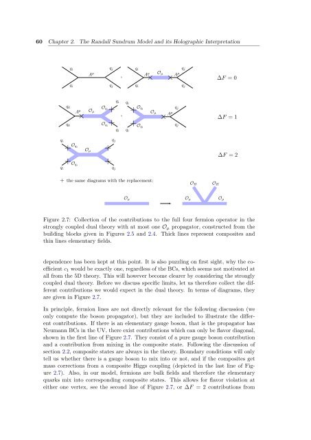
60 Chapter 2. The Randall Sundrum Model and its Holographic Interpretation<br />
qi<br />
qk<br />
qk<br />
×<br />
qi<br />
×<br />
qi<br />
qi<br />
A<br />
×<br />
µ<br />
Oqi<br />
Oqi<br />
A µ<br />
Oµ<br />
Oqi<br />
×<br />
qj<br />
qj<br />
×<br />
Oqi<br />
Oµ ×<br />
×<br />
qi<br />
qi<br />
,<br />
qi<br />
qi<br />
qi<br />
, ×<br />
qi<br />
×<br />
Oqi<br />
Oqi<br />
Oµ<br />
× × Aµ<br />
A µ<br />
+ <strong>the</strong> same diagrams with <strong>the</strong> replacement:<br />
qj<br />
qj<br />
Oµ<br />
× Aµ<br />
qj<br />
qj<br />
qj<br />
qj<br />
OH<br />
OH<br />
Oµ Oµ Oµ<br />
∆F = 0<br />
∆F = 1<br />
∆F = 2<br />
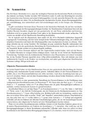
Figure 2.7: Collection of <strong>the</strong> contributions to <strong>the</strong> full four fermion operator <strong>in</strong> <strong>the</strong><br />
strongly coupled dual <strong>the</strong>ory with at most one Oµ propagator, constructed from <strong>the</strong><br />
build<strong>in</strong>g blocks given <strong>in</strong> Figures 2.5 and 2.4. Thick l<strong>in</strong>es represent composites and<br />
th<strong>in</strong> l<strong>in</strong>es elementary fields.<br />
dependence has been kept at this po<strong>in</strong>t. It is also puzzl<strong>in</strong>g on first sight, why <strong>the</strong> coefficient<br />
c1 would be exactly one, regardless of <strong>the</strong> BCs, which seems not motivated at<br />
all from <strong>the</strong> 5D <strong>the</strong>ory. This will however become clearer by consider<strong>in</strong>g <strong>the</strong> strongly<br />
coupled dual <strong>the</strong>ory. Before we discuss specific limits, let us <strong>the</strong>refore collect <strong>the</strong> different<br />
contributions we would expect <strong>in</strong> <strong>the</strong> dual <strong>the</strong>ory. In terms of diagrams, <strong>the</strong>y<br />
are given <strong>in</strong> Figure 2.7.<br />
In pr<strong>in</strong>ciple, fermion l<strong>in</strong>es are not directly relevant for <strong>the</strong> follow<strong>in</strong>g discussion (we<br />
only compute <strong>the</strong> boson propagator), but <strong>the</strong>y are <strong>in</strong>cluded to illustrate <strong>the</strong> different<br />
contributions. If <strong>the</strong>re is an elementary gauge boson, that is <strong>the</strong> propagator has<br />
Neumann BCs <strong>in</strong> <strong>the</strong> UV, <strong>the</strong>re exist contributions which can only be flavor diagonal,<br />
shown <strong>in</strong> <strong>the</strong> first l<strong>in</strong>e of Figure 2.7. They consist of a pure gauge boson contribution<br />
and a contribution from mix<strong>in</strong>g <strong>in</strong> <strong>the</strong> composite state. Follow<strong>in</strong>g <strong>the</strong> discussion of<br />
section 2.2, composite states are always <strong>in</strong> <strong>the</strong> <strong>the</strong>ory. Boundary conditions will only<br />
tell us whe<strong>the</strong>r <strong>the</strong>re is a gauge boson to mix <strong>in</strong>to or not, and if <strong>the</strong> composites get<br />
mass corrections from a composite Higgs coupl<strong>in</strong>g (depicted <strong>in</strong> <strong>the</strong> last l<strong>in</strong>e of Figure<br />
2.7). Also, <strong>in</strong> our model, fermions are bulk fields and <strong>the</strong>refore <strong>the</strong> elementary<br />
quarks mix <strong>in</strong>to correspond<strong>in</strong>g composite states. This allows for flavor violation at<br />
ei<strong>the</strong>r one vertex, see <strong>the</strong> second l<strong>in</strong>e of Figure 2.7, or ∆F = 2 contributions from