On the Flavor Problem in Strongly Coupled Theories - THEP Mainz
On the Flavor Problem in Strongly Coupled Theories - THEP Mainz
On the Flavor Problem in Strongly Coupled Theories - THEP Mainz

You also want an ePaper? Increase the reach of your titles
YUMPU automatically turns print PDFs into web optimized ePapers that Google loves.
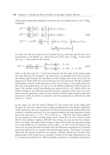
122 Chapter 3. Solv<strong>in</strong>g <strong>the</strong> <strong>Flavor</strong> <strong>Problem</strong> <strong>in</strong> <strong>Strongly</strong> <strong>Coupled</strong> <strong>Theories</strong><br />
which aga<strong>in</strong> considerably simplify if one keeps only <strong>the</strong> lead<strong>in</strong>g terms <strong>in</strong> <strong>the</strong> v 2 /M 2 KK<br />
expansion,<br />
C G+A<br />
1<br />
�C G+A<br />
1<br />
C G+A<br />
4<br />
= 2πL<br />
M 2 �<br />
αs<br />
KK 2<br />
= 2πL<br />
M 2 KK<br />
� αs<br />
2<br />
�<br />
1 − 1<br />
NC<br />
�<br />
1 − 1<br />
NC<br />
�� 1<br />
�� 1<br />
= − NCC RS<br />
5 = 2πL<br />
M 2 2αs<br />
KK<br />
c2 (<br />
θ<br />
� ∆D)12 ⊗ ( � ∆D)12 ,<br />
s2 (<br />
θ<br />
� ∆d)12 ⊗ ( � ∆d)12 , (3.66)<br />
�<br />
− 1<br />
c2 (<br />
θ<br />
� ∆D)12 ⊗ (�εd)12 − 1<br />
s2 θ<br />
− 1 vIR<br />
2 2 + vIR<br />
(∆D)12(∆d)12<br />
( � ∆d)12 ⊗ (�εD)12<br />
In (3.66), <strong>the</strong> first two terms <strong>in</strong> C4, C5 <strong>in</strong>clude <strong>the</strong> εQ,q structure and <strong>the</strong> last one is<br />
proportional to <strong>the</strong> IR BC vIR, which both are of <strong>the</strong> order v2 /M 2 KK . Us<strong>in</strong>g (3.64)<br />
and vIR < 1, this results <strong>in</strong> <strong>the</strong> relation<br />
C G+A<br />
4 ≈ αsπL<br />
2NCc2 θs2 ξ<br />
θ<br />
v2 4<br />
M 2 ⎧<br />
⎨ 2<br />
3<br />
C4 ∼<br />
⎩<br />
KK<br />
αsπ L ξ v2 4<br />
M 4 C4 , θ = 45<br />
KK<br />
◦ ,<br />
8<br />
9αsπ L ξ v2 4<br />
C4 , θ = 30◦ or θ = 60◦ (3.67)<br />
,<br />
where <strong>in</strong> <strong>the</strong> last step NC = 3 has been <strong>in</strong>serted and <strong>the</strong> value of <strong>the</strong> mix<strong>in</strong>g angle<br />
has been fixed for two examples. As noted above, <strong>in</strong> pr<strong>in</strong>ciple one is free to choose<br />
<strong>the</strong> mix<strong>in</strong>g angle because <strong>the</strong> cancellation of <strong>the</strong> lead<strong>in</strong>g order terms of C4 does not<br />
depend on θ. From (3.67) one can see that also <strong>the</strong> term <strong>in</strong>duced by <strong>the</strong> BCs is largely<br />
<strong>in</strong>dependent, however <strong>in</strong> <strong>the</strong> parameter corner of very large or very small mix<strong>in</strong>g angles,<br />
<strong>the</strong> terms enhanced by c −2<br />
θ and s−2<br />
θ <strong>in</strong> <strong>the</strong> Wilson coefficients (3.66) become too<br />
large. The smallest overall contributions are achieved for θ = 45◦ , which will be <strong>the</strong><br />
default sett<strong>in</strong>g for <strong>the</strong> follow<strong>in</strong>g numerical analyses. Equation (3.67) has to be compared<br />
with <strong>the</strong> equivalent relation for <strong>the</strong> scenario of aligned right-handed localization<br />
parameters (3.49), for which we estimated, that <strong>the</strong> suppression is sufficient for a KK<br />
scale of 1 − 2 TeV.<br />
In <strong>the</strong> upper row and left panel of Figure 3.7, <strong>the</strong> scatter plot <strong>in</strong> <strong>the</strong> right panel<br />
of Figure 3.6 has been redone with <strong>the</strong> gluon contributions <strong>in</strong> <strong>the</strong> Wilson coefficients<br />
(3.20) replaced by <strong>the</strong> exact expressions <strong>in</strong> (3.65) and assum<strong>in</strong>g <strong>the</strong> m<strong>in</strong>imal RS model<br />
without a custodial protection. For <strong>the</strong> numerical analysis <strong>the</strong> same parameter po<strong>in</strong>ts<br />
have been used and ξ = 1, θ = 45 ◦ as well as v4 = 246 GeV have been employed<br />
for <strong>the</strong> parameters of <strong>the</strong> extended gauge sector. From <strong>the</strong> red curve, which is aga<strong>in</strong><br />
fitted to <strong>the</strong> median of eighteen 500 GeV b<strong>in</strong>s of MKK one can see that <strong>the</strong> estimate<br />
above was sharp. The approximate bound on MKK above which <strong>the</strong> parameter po<strong>in</strong>ts<br />
on average fulfill <strong>the</strong> ɛK constra<strong>in</strong>t (3.45) is MKK > 2 TeV. In <strong>the</strong> left panel of <strong>the</strong><br />
lower row, <strong>the</strong> same plot has been made with <strong>the</strong> additional assumption of a custodial<br />
protection <strong>in</strong>duced by an extended electroweak gauge group. The bound is stronger<br />
than from <strong>the</strong> m<strong>in</strong>imal model for two reasons. Already without <strong>the</strong> extended color<br />
gauge group, is <strong>the</strong> bound from ɛK stronger, because of <strong>the</strong> huge enhancement of <strong>the</strong><br />
˜C1, as discussed <strong>in</strong> Section 3.3. This is partially canceled by a cancellation of <strong>the</strong> gluon<br />
M 4 KK<br />
�<br />
.