On the Flavor Problem in Strongly Coupled Theories - THEP Mainz

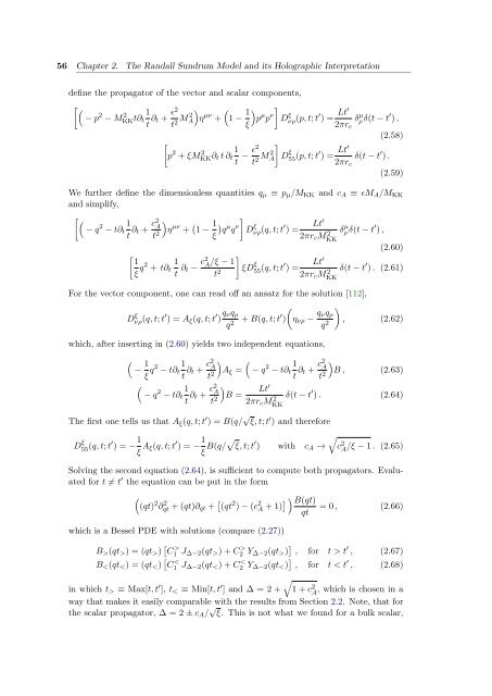
56 Chapter 2. The Randall Sundrum Model and its Holographic Interpretation
define the propagator of the vector and scalar components,
�� − p 2 − M 2 1
KKt∂t
t ∂t + ɛ2
t2 M 2 �
A η µν �
+ 1 − 1
�
p
ξ
µ p ν
�
D ξ νρ(p, t; t ′ ) = Lt′
2πrc
�
p 2 + ξM 2 KK∂t t ∂t
1
t
δ µ ρ δ(t − t ′ ) ,
(2.58)
ɛ2
−
t2 M 2 �
A D ξ
55 (p, t; t′ ) = Lt′
δ(t − t
2πrc
′ ) .
(2.59)
We further define the dimensionless quantities qµ ≡ pµ/MKK and cA ≡ ɛMA/MKK
and simplify,
� �
− q 2 1
− t∂t
t ∂t + c2 A
t2 �
η µν + � 1 − 1
ξ
�
� µ ν
q q
D ξ νρ(q, t; t ′ ) =
�
1
ξ q2 1
+ t∂t
t ∂t − c2 A /ξ − 1
t2 �
ξD ξ
55 (q, t; t′ ) =
D ξ νρ(q, t; t ′ ) = Aξ(q, t; t ′ ) qνqρ
q 2 + B(q, t; t′ )
Lt′
2πrcM 2 δ
KK
µ ρ δ(t − t ′ ) ,
Lt′
2πrcM 2 KK
ηνρ − qνqρ
q 2
(2.60)
δ(t − t ′ ) . (2.61)
For the vector component, one can read off an ansatz for the solution [112],
� �
, (2.62)
which, after inserting in (2.60) yields two independent equations,
�
− 1
ξ q2 1
− t∂t
t ∂t + c2 A
t2 � �
Aξ = − q 2 1
− t∂t
t ∂t + c2 A
t2 �
B , (2.63)
�
�
Lt
B =
′
δ(t − t ′ ) . (2.64)
− q 2 1
− t∂t
t ∂t + c2 A
t2 2πrcM 2 KK
The first one tells us that Aξ(q, t; t ′ ) = B(q/ √ ξ, t; t ′ ) and therefore
D ξ
55 (q, t; t′ ) = − 1
ξ Aξ(q, t; t ′ ) = − 1
ξ B(q/�ξ, t; t ′ �
) with cA → c2 A /ξ − 1 . (2.65)
Solving the second equation (2.64), is sufficient to compute both propagators. Evaluated
for t �= t ′ the equation can be put in the form
�
(qt) 2 ∂ 2 qt + (qt)∂qt + � (qt 2 ) − (c 2 A + 1) � � B(qt)
= 0 , (2.66)
qt
which is a Bessel PDE with solutions (compare (2.27))
B>(qt>) = (qt>) � C > 1 J∆−2(qt>) + C > 2 Y∆−2(qt>) � , for t > t ′ , (2.67)
B