On the Flavor Problem in Strongly Coupled Theories - THEP Mainz

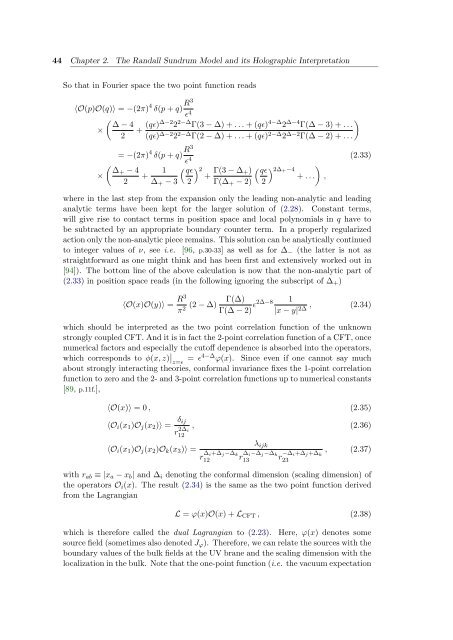
44 Chapter 2. The Randall Sundrum Model and its Holographic Interpretation
So that in Fourier space the two point function reads
〈O(p)O(q)〉 = −(2π) 4 δ(p + q) R3
ɛ4 �
∆ − 4
×
2 + (qɛ)∆−222−∆Γ(3 − ∆) + . . . + (qɛ) 4−∆2∆−4Γ(∆ − 3) + . . .
(qɛ) ∆−222−∆Γ(2 − ∆) + . . . + (qɛ) 2−∆2∆−2 �
Γ(∆ − 2) + . . .
= −(2π) 4 δ(p + q) R3
ɛ4 �
∆+ − 4 1
�
qɛ
× +
2 ∆+ − 3 2
� 2
+ Γ(3 − ∆+)
Γ(∆+ − 2)
�
qɛ
� �
2∆+−4
+ . . . ,
2
(2.33)
where in the last step from the expansion only the leading non-analytic and leading
analytic terms have been kept for the larger solution of (2.28). Constant terms,
will give rise to contact terms in position space and local polynomials in q have to
be subtracted by an appropriate boundary counter term. In a properly regularized
action only the non-analytic piece remains. This solution can be analytically continued
to integer values of ν, see i.e. [96, p.30-33] as well as for ∆− (the latter is not as
straightforward as one might think and has been first and extensively worked out in
[94]). The bottom line of the above calculation is now that the non-analytic part of
(2.33) in position space reads (in the following ignoring the subscript of ∆+)
〈O(x)O(y)〉 = R3 Γ(∆)
(2 − ∆)
π2 Γ(∆ − 2) ɛ2∆−8
1
, (2.34)
|x − y| 2∆
which should be interpreted as the two point correlation function of the unknown
strongly coupled CFT. And it is in fact the 2-point correlation function of a CFT, once
numerical factors and especially the cutoff dependence is absorbed into the operators,
which corresponds to φ(x, z) � � z=ɛ = ɛ 4−∆ ϕ(x). Since even if one cannot say much
about strongly interacting theories, conformal invariance fixes the 1-point correlation
function to zero and the 2- and 3-point correlation functions up to numerical constants
[89, p.11f.],
〈O(x)〉 = 0 , (2.35)
〈Oi(x1)Oj(x2)〉 = δij
r 2∆i
12
, (2.36)
λijk
〈Oi(x1)Oj(x2)Ok(x3)〉 =
r ∆i+∆j−∆k
12
r ∆i−∆j−∆k
13 r −∆i+∆j+∆k
23
, (2.37)
with rab ≡ |xa − xb| and ∆i denoting the conformal dimension (scaling dimension) of
the operators Oi(x). The result (2.34) is the same as the two point function derived
from the Lagrangian
L = ϕ(x)O(x) + LCFT , (2.38)
which is therefore called the dual Lagrangian to (2.23). Here, ϕ(x) denotes some
source field (sometimes also denoted Jϕ). Therefore, we can relate the sources with the
boundary values of the bulk fields at the UV brane and the scaling dimension with the
localization in the bulk. Note that the one-point function (i.e. the vacuum expectation