On the Flavor Problem in Strongly Coupled Theories - THEP Mainz

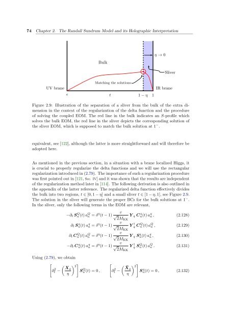
74 Chapter 2. The Randall Sundrum Model and its Holographic Interpretation
Bulk
Sliver
Matching the solutions
UV brane IR brane
ɛ t 1 − η 1
η → 0
Figure 2.9: Illustration of the separation of a sliver from the bulk of the extra dimension
in the context of the regularization of the delta function and the procedure
of solving the coupled EOM. The red line in the bulk indicates an S-profile which
solves the bulk EOM, the red line in the sliver depicts the corresponding solution of
the sliver EOM, which is supposed to match the bulk solution at 1 − .
equivalent, see [122], although the latter is more straightforward and will therefore be
adopted here.
As mentioned in the previous section, in a situation with a brane localized Higgs, it
is crucial to properly regularize the delta functions and we will use the rectangular
regularization introduced in (2.79). The importance of such a regularization procedure
was first pointed out in [121, Sec. IV] and it was shown that the results are independent
of the regularization method later in [114]. The following derivation is also outlined in
the appendix of the latter reference. The regularized delta function effectively divides
the bulk into two regions, t ∈ [0, 1 − η] and a small sliver t ∈ [1 − η, 1], see Figure 2.9.
The solution in the sliver will generate the proper BCs for the bulk solutions at 1 − .
In the sliver, only the following terms in the EOM are relevant,
−∂t S Q n (t) a Q n = δ η (t − 1)
∂t S q n(t) a q n = δ η (t − 1)
∂t C Q n (t) a Q n = δ η (t − 1)
−∂t C q n(t) a q n = δ η (t − 1)
Using (2.79), we obtain
�
∂ 2 � � �
2
Xq
t − S
η
Q n (t) = 0 ,
�
v
√ Y q C
2MKK
q n(t) a q n , (2.128)
v
√ Y
2MKK
† q C Q n (t) a Q n , (2.129)
v
√ Y q S
2MKK
q n(t) a q n , (2.130)
v
√ Y
2MKK
† q S Q n (t) a Q n . (2.131)
∂ 2 t −
� � �
¯Xq
2
S
η
q n(t) = 0 , (2.132)