On the Flavor Problem in Strongly Coupled Theories - THEP Mainz
On the Flavor Problem in Strongly Coupled Theories - THEP Mainz
On the Flavor Problem in Strongly Coupled Theories - THEP Mainz

Create successful ePaper yourself
Turn your PDF publications into a flip-book with our unique Google optimized e-Paper software.
2.3. Profiles of Gauge Bosons 61<br />
pure composite exchange, which can be found <strong>in</strong> <strong>the</strong> third l<strong>in</strong>e of Figure 2.7. Keep <strong>in</strong><br />
m<strong>in</strong>d, that <strong>the</strong>se diagrams are flavor-diagonal <strong>in</strong> Figure 2.7, but not flavor universal,<br />
which will lead to <strong>the</strong> described flavor violation after rotation <strong>in</strong>to <strong>the</strong> basis <strong>in</strong> which<br />
<strong>the</strong> Yukawa matrices are diagonal. Also, <strong>the</strong> diagrams <strong>in</strong> <strong>the</strong> second and third l<strong>in</strong>e<br />
of Figure 2.7 can give flavor conserv<strong>in</strong>g and ∆F = 1 contributions as well, <strong>the</strong> right<br />
hand side only denotes <strong>the</strong> maximal number of vertices at which flavor violation can<br />
occur simultaneously. Fur<strong>the</strong>r diagrams can be constructed through additional mix<strong>in</strong>g<br />
from composites <strong>in</strong>to <strong>the</strong> elementary states and back. However, each additional Oµ<br />
propagator carries ano<strong>the</strong>r factor M −2<br />
KK and will <strong>the</strong> correspond<strong>in</strong>g terms will thus be<br />
suppressed.<br />
An <strong>in</strong>terest<strong>in</strong>g result of this <strong>the</strong>sis is, that we are able to assign diagrams <strong>in</strong> <strong>the</strong> dual<br />
<strong>the</strong>ory to <strong>the</strong> different contributions of (2.82), by systematically consider<strong>in</strong>g different<br />
BCs. In <strong>the</strong> follow<strong>in</strong>g, <strong>the</strong> respective BCs and <strong>the</strong> contribut<strong>in</strong>g diagrams are<br />
shown on <strong>the</strong> left hand side. Also, after perform<strong>in</strong>g <strong>the</strong> limits for <strong>the</strong> respective BCs,<br />
ɛ-suppressed factors will be omitted and <strong>the</strong> results are given <strong>in</strong> Feynman-’t Hooft<br />
gauge, ξ = 1. Let us start with <strong>the</strong> “cleanest” scenario.<br />
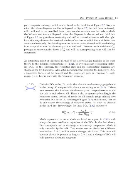
(DN) Dirichlet BCs <strong>in</strong> <strong>the</strong> UV imply, that <strong>the</strong>re is no elementary gauge boson<br />
<strong>in</strong> <strong>the</strong> <strong>the</strong>ory. Consequentially, <strong>the</strong>re is no mix<strong>in</strong>g as <strong>in</strong> (2.41). If <strong>the</strong>re<br />
were no composite fermions, <strong>the</strong> elementary and composite sector would<br />
not talk to each o<strong>the</strong>r at all. There is also no symmetry break<strong>in</strong>g <strong>in</strong> <strong>the</strong><br />
composite sector, because all fields (for all possible gauge <strong>in</strong>dices) have<br />
Neumann BCs <strong>in</strong> <strong>the</strong> IR. Referr<strong>in</strong>g to Figure (2.7), that means, that we<br />
do only expect <strong>the</strong> exchange of composite states, i.e. only <strong>the</strong> diagram<br />
<strong>in</strong> <strong>the</strong> third l<strong>in</strong>e. Interest<strong>in</strong>gly, for <strong>the</strong>se BCs, (2.82) reduces to<br />
D ξ=1<br />
µν (q, t; t ′ ) = ηµν L<br />
4πrc M 2 t<br />
KK<br />
2 < , (2.84)<br />
which represents <strong>the</strong> term which we found to appear <strong>in</strong> (2.82) with<br />
always <strong>the</strong> same coefficient regardless of <strong>the</strong> BCs. In <strong>the</strong> dual <strong>the</strong>ory,<br />
this corresponds to <strong>the</strong> exchange of exclusively composites, which is<br />
only controlled by <strong>the</strong> bulk. That means, one can check that a different<br />
localization, ∆ �= 3, will <strong>in</strong> general change this factor. This term will<br />
however always be present as long as ∆ = 3 and a change of BCs will<br />
only generate additional diagrams.