Workshop proceeding - final.pdf - Faculty of Information and ...

3. Dynamic model for approaching targets
As concerns the choice of target dynamic model, it’s tied to the adapted tracking coordinate system.
The most natural coordinate is the Cartesian coordinate. In a Cartesian system, the target state is
described by ( x, xyy , , ) T x y
x& y&
is the velocity vector.
Φ = & & , where ( , ) k
k
k
is the target’s position; ( , ) k
2 2
Velocity vector can be described by speed and heading pair (, v α , where v = x& + y& ,
and arctan ( x / y)
α = & & .
However, in the situation under our consideration, the measurements are the reflected power on the
ambiguous range-Doppler (i.e., range-apparent Doppler) grid. Thus, the choice of the Cartesian
coordinate requires a nonlinear transformation which results in increased complexity. It’s of interest to
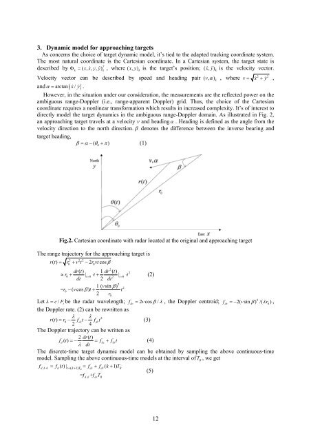
directly model the target dynamics in the ambiguous range-Doppler domain. As illustrated in Fig. 2,
an approaching target travels at a velocity v and headingα . Heading is defined as the angle from the
velocity direction to the north direction. β denotes the difference between the inverse bearing and
target heading,
β = α − ( θ + π)
(1)
0
) k
Fig.2. Cartesian coordinate with radar located at the original and approaching target
The range trajectory for the approaching target is
2 2 2
rt () = r + vt −2rvtcosβ
0 0
2
dr() t 1 dr () t 2
r0 |
t=
0
t |
2 t= 0
t (2)
≈ + ⋅ + ⋅
dt 2 dt
2
1( vsin β ) 2
= r0
− ( vcos β ) t+
t
2 r0
2
Let λ = c/ Ft
be the radar wavelength; fdc
= 2vcos β / λ , the Doppler centroid; fdr
=− 2( vsin β ) /( λr0
) ,
the Doppler rate. (2) can be rewritten as
λ λ 2
rt () = r0
− fdct− fdrt
(3)
2 4
The Doppler trajectory can be written as
2 dr( t)
fd()
t =− = f dc
+ f dr
t (4)
λ dt
The discrete-time target dynamic model can be obtained by sampling the above continuous-time
model. Sampling the above continuous-time models at the interval ofT R
, we get
fdk , + 1
= fd()| t
t= ( k+
1) T
= f ( 1)
R dc+ fdr k+
TR
(5)
= f + f T
dk , dr R
12