Workshop proceeding - final.pdf - Faculty of Information and ...

k
k k k
( ) p(
p Ζ | X , B = ∏ zk | x
k,
b
k)
(27)
k = 1
k
k
given the target trajectory X = ( x1, x2,..., xk
) and nuisance parameter B = ( b1
,..., b k
).
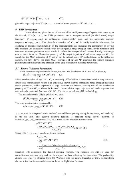
5. TBD Procedures
In our situation, given the set of unthresholded ambiguous range-Doppler data maps up to
k
the k th visit, Z = ( z ,..., 1
z
k ) , the TBD procedures aim to compute optimal (in MAP sense) target
k
trajectory X = ( x1, x2,..., xk
) in ambiguous range-Doppler map, and its ambiguity number
k
k k
sequence Μ = ( m1
,..., m k
) . The close-form solution of X , Μ is hardly feasible. Moreover, the
k
existence of nuisance parameters, B in the measurements also increases the complexity of solving
this problem. An exhaustive search over the ambiguous range-Doppler maps, mode parameter and
unknown nuisance parameter space results in unbearable computational burden. Luckily, advantage
k
k
can be taken from the Markovian property of the target trajectory X and mode sequence Μ , the
k
k
search for the MAP estimates of X and Μ can be solved using DP methodology. In the following
k
k
section, we first derive the joint MAP estimates of X and Μ assuming the known nuisance
parameters and then extend the approach to the case of unknown nuisance parameters.
5.1 Known Nuisance Parameters
k
k
When the nuisance parameter is known, the joint MAP estimates of X and Μ is given by
ˆ k
( , ˆ k k k k
X Μ ) = arg max p( X , Μ | Z ) (28)
k X , Μ
k
k k k
Direct maximization of p( X , Μ | Z ) is extremely difficult since a close-form solution may not exist.
Brute-force maximization results in an exhaustive search over the ambiguous range-Doppler maps and
mode parameters, which represents a huge computation burden. Making use of the Markovian
k
k
property of X and Μ , as shown in Section 3, the search for target trajectory and mode sequence that
k k k
maximize the posteriori function p( X , Μ | Z ) can be solved using DP methodology.
The maximization in (28) is split into two parts
ˆ k ˆ k k k k
( X , Μ ) = argmax
⎡
max p( , | )
⎤
, k 1 k 1
k m ⎢
X M Z
x − −
k⎣X , M
⎥
(29)
⎦
The inner maximization is denoted by
( , ) max ( k , k | k
I x m = p X M Z ) (30)
k k k
,
k−1 k−1
X M
Ik( xk, mk)
can be interpreted as the merit of the candidate trajectory ending in any state xk
and mode mk
at the kth visit. The desired iterative relation is obtained using Bayes’ theorem to
express Ik+ 1( x
k+ 1,
mk+
1) in terms of Ik( x
k, mk)
. From Bayes’ theorem it follows that
k+ 1 k+ 1 k+
1
p( X , Μ | Z )
p( zk+ 1| xk+ 1) p( xk+ 1| xk, mk) p( mk+
1| mk, xk)
(31)
k k k
= p( X , Μ | Z )
k
p( zk+
1
| Z )
Using (31), Ik+ 1( x
k+ 1,
mk+
1)
can be written in the form
Ik+ 1( xk+ 1, mk+
1)
k+ 1 k+ 1 k+
1
= max p( X , Μ | Z )
(32)
X
k
, Mk
⎧p( zk+ 1| xk+ 1) p( xk+ 1| xk, mk) p( mk+
1| mk, xk)
⎫
= max ⎨ Ik( xk, mk)
k,
m
k
⎬
x k⎩
p( zk+
1
| Z )
⎭
k
Equation (32) constitutes the desired iterative relation. The function p ( zk
+ 1
| Z ) is used for
normalization purposes only and can be dropped without affecting the maximizer. The probability
density p ( z )
k+ 1
| x
k+
1
is obtained from(26). Working with the natural logarithm of (32), we transform
the merit function into an additive rather than a multiplicative function.
16