Workshop proceeding - final.pdf - Faculty of Information and ...
Workshop proceeding - final.pdf - Faculty of Information and ...
Workshop proceeding - final.pdf - Faculty of Information and ...

You also want an ePaper? Increase the reach of your titles
YUMPU automatically turns print PDFs into web optimized ePapers that Google loves.
mean δ<br />
ij<br />
= 50 Hz <strong>and</strong> variance Σ<br />
ij<br />
= 16 , denoted byδij<br />
N ( δij<br />
;50,16), <strong>and</strong> then, as discussed in Section<br />
3, the state-dependent ambiguity number transition probability is<br />
⎧Φ( Cx<br />
ij k<br />
−δij ; Σ<br />
ij ) if j = i<br />
⎪<br />
πij ( xk ) = ⎨1 −Φ( Cijx k<br />
−δij; Σ<br />
ij ) if j = i−1<br />
(52)<br />
⎪<br />
0 else<br />
⎪⎩<br />
A maximum target velocity v<br />
max<br />
= 3Mach is assumed in our simulation.<br />
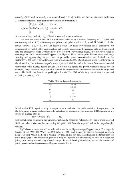
We consider here a low PRF surveillance radar using a carrier frequency <strong>of</strong> 1.2 GHz <strong>and</strong><br />
transmitting trains <strong>of</strong> N<br />
d<br />
= 64 rectangular pulses with pulse width τ = 1.2 μs<br />
<strong>and</strong> PRF=860 Hz. Radar<br />
revisit interval is T<br />
R<br />
= 4 s . For the reader’s sake, the main surveillance radar parameters are<br />
summarized in Table I .After discretization <strong>and</strong> Doppler processing, the received data are transformed<br />
into the ambiguous range-Doppler maps. For low PRF surveillance radars, the measured range is<br />
unambiguous while the measured Doppler is ambiguous. Since we are primarily concerned with early<br />
warning <strong>of</strong> approaching targets, the range cells under consideration are limited to the<br />
furthest N<br />
r<br />
= 256 cells. Thus, after each visit, we obtained a 256× 64 ambiguous range-Doppler map. In<br />
the simulation, the unknown target’s power u k<br />
at each visit is r<strong>and</strong>omly drawn from an exponential<br />
distribution with average return power u . Note that we ignore the power variation caused by the<br />
changing range since the range variation is small in comparison to the distance between the target <strong>and</strong><br />
radar. The SNR is defined in range-Doppler domain. The SNR <strong>of</strong> the target at kth visit is expressed<br />
2<br />
as (SNR) = 10log( u / σ ) .<br />
k<br />
k<br />
Table I Radar System Parameters<br />
It’s clear that SNR experienced by the target varies at each visit due to the variation <strong>of</strong> target power. In<br />
the following, in order to characterize the detection performance <strong>of</strong> the proposed TBD algorithms, we<br />
define an average SNR as<br />
2<br />
SNR = 10log( u / σ ) (53)<br />
Notice that, since we assume the number <strong>of</strong> coherently processed pulses N<br />
d<br />
= 64 , the average received<br />
SNR per pulse is obtained by subtracting 10log 64 18dB from the reported values in range-Doppler<br />
domain.<br />
Fig.7 shows a mesh plot <strong>of</strong> the reflected power in ambiguous range-Doppler maps. The target is<br />
located at cell (231, 14). When the SNR is high (13dB) <strong>and</strong> it’s easy to discern the target as a high<br />
peak (Fig.7(a)). When the SNR is relative low (10dB), it’s not easy to distinguish the target from the<br />
noise (Fig.7(b)). TBD procedures provide a way to improve the detestability <strong>of</strong> low SNR target by<br />
jointly processing several range-Doppler maps. In the following simulation, we set the number <strong>of</strong><br />
jointly processed ambiguous range-Doppler maps to K = 6 .<br />
21