Workshop proceeding - final.pdf - Faculty of Information and ...
Workshop proceeding - final.pdf - Faculty of Information and ...
Workshop proceeding - final.pdf - Faculty of Information and ...

Create successful ePaper yourself
Turn your PDF publications into a flip-book with our unique Google optimized e-Paper software.
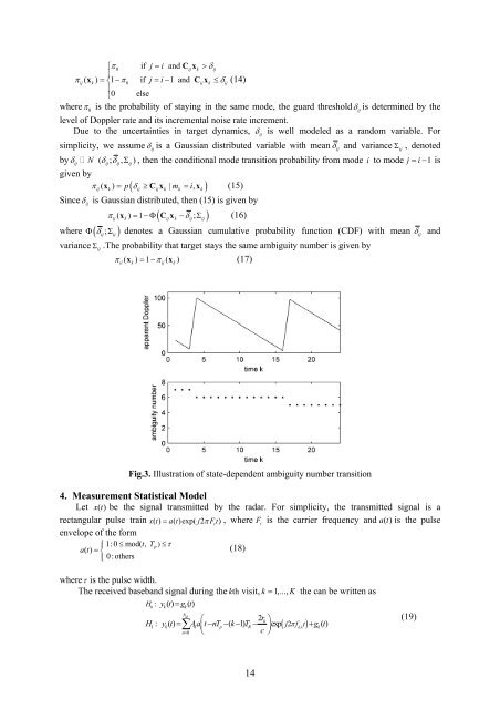
⎧π0<br />
if j = i <strong>and</strong> Cx<br />
ij k<br />
> δij<br />
⎪<br />
π<br />
ij<br />
( xk ) = ⎨1 − π0<br />
if j = i−1 <strong>and</strong> Cijx k<br />
≤δij<br />
(14)<br />
⎪<br />
⎩0 else<br />
whereπ 0<br />
is the probability <strong>of</strong> staying in the same mode, the guard thresholdδ ij<br />
is determined by the<br />
level <strong>of</strong> Doppler rate <strong>and</strong> its incremental noise rate increment.<br />
Due to the uncertainties in target dynamics, δ<br />
ij<br />
is well modeled as a r<strong>and</strong>om variable. For<br />
simplicity, we assume δ ij<br />
is a Gaussian distributed variable with mean δ ij<br />
<strong>and</strong> variance Σ ij<br />
, denoted<br />
byδ N ( δ ; δ , Σ ), then the conditional mode transition probability from mode i to mode j = i − 1 is<br />
ij ij ij ij<br />
given by<br />
π ( x ) = p δ ≥ C x | m = i,<br />
x<br />
( )<br />
ij k ij ij k k k<br />
(15)<br />
Sinceδ ij<br />
is Gaussian distributed, then (15) is given by<br />
( δ )<br />
π ( x ) = 1 −Φ C x − ; Σ (16)<br />
ij k ij k ij ij<br />
where Φ( δ ij<br />
; Σ ij ) denotes a Gaussian cumulative probability function (CDF) with mean δ ij<br />
<strong>and</strong><br />
variance<br />
Σ ij<br />
.The probability that target stays the same ambiguity number is given by<br />
π ( x ) = 1 −π<br />
( x )<br />
(17)<br />
ii k ij k<br />
Fig.3. Illustration <strong>of</strong> state-dependent ambiguity number transition<br />
4. Measurement Statistical Model<br />
Let x()<br />
t be the signal transmitted by the radar. For simplicity, the transmitted signal is a<br />
rectangular pulse train x() t = a()exp( t j2 π Ft t ), where F t<br />
is the carrier frequency <strong>and</strong> at () is the pulse<br />
envelope <strong>of</strong> the form<br />
⎧⎪ 1:0 ≤mod( t,<br />
T p ) ≤τ<br />
(18)<br />
at () = ⎨<br />
⎪⎩ 0:others<br />
whereτ is the pulse width.<br />
The received baseb<strong>and</strong> signal during the kth<br />
visit, k = 1,..., K the can be written as<br />
H : y () t = g () t<br />
0<br />
k<br />
k<br />
Nd<br />
⎛<br />
2r<br />
k ⎞<br />
H1<br />
: yk() t = ∑Aa k ⎜t−nTp−( k−1) TR− exp ( j2π<br />
f t<br />
, ) + g ()<br />
dk k<br />
t<br />
n=<br />
0<br />
c<br />
⎟<br />
⎝<br />
⎠<br />
(19)<br />
14