Workshop proceeding - final.pdf - Faculty of Information and ...

optical image Im Oe ,
Im Oek,l
is an image located in (k,l)th of the image Im Oe and its size is the same as
image Im IRe , σ k,l and σ IR are the standard deviation of the corresponding images respectively.
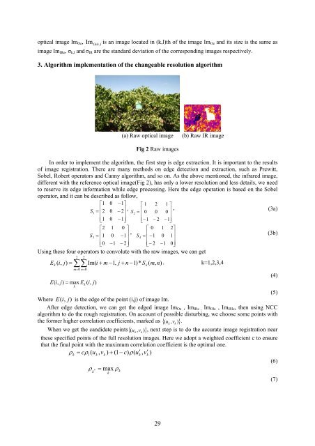
3. Algorithm implementation of the changeable resolution algorithm
(a) Raw optical image
(b) Raw IR image
Fig 2 Raw images
In order to implement the algorithm, the first step is edge extraction. It is important to the results
of image registration. There are many methods on edge detection and extraction, such as Prewitt,
Sobel, Robert operators and Canny algorithm, and so on. As the above mentioned, the infrared image,
different with the reference optical image(Fig 2), has only a lower resolution and less details, we need
to reserve its edge information while edge processing. Here the edge operation is based on the Sobel
operator, and it can be described as follow,
⎡1
0 −1⎤
⎡ 1 2 1 ⎤
S =
⎢ ⎥
⎢
2 0 − 2 , , (3a)
1
⎥ S
⎢
⎥
2
=
⎢
0 0 0
⎥
⎢⎣
1 0 −1⎥⎦
⎢⎣
−1
− 2 −1⎥⎦
⎡2
1 0 ⎤ ⎡ 0 1 2⎤
S =
⎢ ⎥
⎢
1 0 −1
,
3
⎥
S
⎢ ⎥
(3b)
4
=
⎢
−1
0 1
⎥
⎢⎣
0 −1
− 2⎥⎦
⎢⎣
− 2 −1
0⎥⎦
Using these four operators to convolute with the raw images, we can get
2
2
∑∑
E ( i,
j)
= Im( i + m −1,
j + n −1)*
S ( m,
n)
. k=1,2,3,4
k
m= 0 n=
0
E( i,
j)
= max E ( i,
j)
k
k
k
(5)
Where E( i,
j)
is the edge of the point (i,j) of image Im.
After edge detection, we can get the edged image Im Oe , Im IRe , Im Ole , Im IRle , then using NCC
algorithm to do the rough registration. On account of possible disturbing, we choose some points with
the former higher correlation coefficients, marked as {( u
k
, vk
)}.
When we get the candidate points{ ( u k
, v , next step is to do the accurate image registration near
k
)}
these specified points of the full resolution images. Here we adopt a weighted coefficient c to ensure
that the final point with the maximum correlation coefficient is the optimal one.
ρ
k
= c ρl
( uk
, vk
) + (1 − c)
ρ(
u′
k
, v′
k
)
(6)
ρ max ρ
* =
k
k
k
(4)
(7)
29