The mechanical effects of short-circuit currents in - Montefiore

More documents

Recommendations

Info

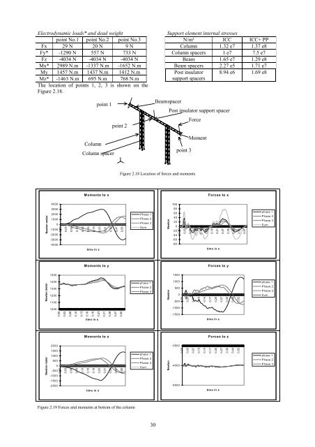
Electrodynamic loads* and dead weight point No.1 point No.2 point No.3 Fx 29 N 20 N 9 N Fy* -1290 N 557 N 733 N Fz -4034 N -4034 N -4034 N Mx* 2989 N.m -1337 N.m -1652 N.m My 1457 N.m 1437 N.m 1412 N.m Mz* -1463 N.m 695 N.m 768 N.m The location of points 1, 2, 3 is shown on the Figure 2.18. Newton meter Newton meter Newton meter 4000 3000 2000 1000 0 -1000 -2000 -3000 -4000 1500 1400 1300 1200 1100 1000 0,00 0,00 2000 1500 1000 500 0 -500 -1000 -1500 -2000 0,00 0,03 0,03 0,03 0,06 0,06 0,06 0,10 0,10 0,10 0,13 0,13 0,13 Column point 1 Column spacer Moments to x 0,16 0,19 0,23 time in s 0,31 Moments to y 0,16 0,19 0,23 time in s 0,31 Moments to z 0,16 0,19 0,23 time in s 0,39 0,39 point 2 Figure 2.19 Forces and moments at bottom of the column 0,31 0,39 0,47 0,47 0,47 30 Support element internal stresses N/m² ICC ICC+ PP Column 1.32 e7 1.37 e8 Column spacers 1 e7 7.5 e7 Beam 1.65 e7 1.29 e8 Beam spacers 2.27 e5 1.71 e7 Post insulator support spacers 8.94 e6 1.69 e8 Beamspacer Post insulator support spacer point 3 Force Figure 2.18 Location of forces and moments 0,55 0,55 0,55 Phase 1 Phase 2 Phase 3 Sum phase 1 Phase 2 Phase 3 phase 1 Phase 2 Phase 3 Sum Newton Newton Newton 100 80 60 40 20 0 -20 -40 -60 -80 0,00 1500 1000 500 0 -500 -1000 -1500 -3500 -4000 -4500 0,00 0,00 0,03 0,03 0,03 Moment 0,06 0,07 0,07 0,09 0,10 0,10 0,12 0,15 0,14 0,14 Forces to x 0,18 0,21 time in s 0,27 0,35 Forces to y 0,17 0,20 time in s 0,27 0,35 Forces to z 0,17 0,20 time in s 0,27 0,35 0,42 0,44 0,44 0,50 0,52 0,52 0,57 phase 1 Phase 2 Phase 3 Sum phase 1 Phase 2 Phase 3 Sum phase 1 Phase 2 Phase 3
2.3.2. Influence of two busbars a) Introduction Many substations have several busbars in parallel. To handle three-phase or phase to phase faults on 1 or 2 busbars, a special analyses is done in this section to approach the maximum amplitude of stresses to define the withstanding capability of the structures. For example, RTE takes the following fault situation named « transfer situation » into account when only one line is temporarily protected by the « coupling bay » protections : Figure 2.20 Two busbars in parallel An amplification coefficient is introduced which allows one to step from a reference situation to the actual configuration depending on the type of substation (separated or associated phase layout) and of the fault to be analysed. This approach gives also the maximum asymmetry for these cases. b) General considerations The amplitude of the LAPLACE’s force depends on the location of the considered phase, the type of fault and the characteristic of the fault. Phase to phase fault and phase to earth fault Due to the linear properties of the mechanical equations, the maximum of the force corresponding to the maximum asymmetry is obtained when the phase voltage is zero at the beginning of the fault. The amplification coefficients are given below and are without approximation. Three-phase fault If the instant expression of LAPLACE’s force is given by an expression of the type : µ 2π let us suppose that : 0 (2.81) F = . i . ( α. i + β. i + γ . i ) (2.82) K = α. a + β + γ. a = K . e where a = e 2 2 1 j. Φ In this paragraph, Re(K) is the real part of K. 2 3 2π j 3 The maximum force is reached after ½ period and its value is : 31 ) µ 0 F = . Ik′′ . 2π (2.83) ) µ 0 F = . Ik′′ . 2π (2.84) ( 2. κ) ⎛ 2⎛Φ ⎞ 2⎛Φ ⎞⎞ . K . MAX ⎜ ⎜cos ⎜ ⎟, sin ⎜ ⎟ 2 2 ⎟ ⎝ ⎝ ⎠ ⎝ ⎠⎠ 2 2 K + Re( K) ( 2. κ) . 2 −3R X κ = 1. 02 + 0. 98e κ : factor for the calculation of the peak shortcircuit current [Ref 11]. The main steps which allow one to obtain this relation are given in [Ref 99]. The solution to this problem seemingly allows the main situations met to be handled (separated phases and associated phases . . .). The amplification coefficient in this case is not exact because this optimization is done on the force not on the dynamic response of the system. All components defined in paragraph 2.2 of Ref 1 are taken into account same as in the IEC standard. The dynamic behavior can differ likely like for the central busbar for an associated-phase layout in a three-phase fault in comparison with this optimization [Ref 8]. If the reference situation is calculated with an advanced method taking into account time constant and fault clearance time, the amplification coefficient is applied to the maximum Freference. (2.85) ) F = F . xb reference Kxp The tables given below can be used to find the maximum of asymmetry on a bar during a threephase fault on two busbars. This asymmetry is given on phase 1 of the busbar 1. c) Laplace’s force due to the short-circuit There are three possible layouts : - separate-phase layout, - asymmetrical associated-phase layout, - symmetrical associated-phase layout. For the separate-phase layout, the maximum LAPLACE force named reference in Table 2.5 is given by : (2.86) F reference µ 0 = 2π " ( I 2κ ) k1 corresponding to a phase to earth fault in transfer situation. For the associated-phase layouts, the maximum LAPLACE force named reference in Table 2.6 and Table 2.7 is given by : (2.87) F reference µ 0 = 2π d 2 " 2 ( I k 2κ ) 3 d 4 corresponding to a phase to phase fault on one busbar. Both these values can be calculated by advanced methods.
Page 1 and 2: THE MECHANICAL EFFECTS OF SHORT-CIR
Page 3 and 4: 3.7. Special problems .............
Page 5 and 6: 1. INTRODUCTION 1.1. GENERAL PRESEN
Page 7 and 8: The pinch (first maximum) can be ve
Page 9 and 10: 1.3.3.2 Supporting structures Simil
Page 11 and 12: This method allows to state the sho
Page 13 and 14: and becomes the static force in equ
Page 15 and 16: (2.26) M el-pl ⎡ y d/ 2 y = 2⎢
Page 17 and 18: V σ 3 2,5 2 1,5 1 mechanical reson
Page 19 and 20: V F 3 2,5 2 1,5 1 mechanical resona
Page 21 and 22: 1. eigenmode 2. eigenmode 3. eigenm
Page 23 and 24: (2.43) U E max max = 1 2 1 = 2 l
Page 25 and 26: m (2.47) M = σm = Z mσ m dm 2 J w
Page 27 and 28: profiles in Figure 2.14 it follows
Page 29: (2.71) 2 tube tube 4 tube U ∂U
Page 33 and 34: Asymmetrical associated-phase layou
Page 35 and 36: d)Methods used IEC 60865 method : -
Page 37 and 38: Section 3.4 deals with the effects
Page 39 and 40: In Figure 3.5 to Figure 3.8, the ma
Page 41 and 42: Figure 3.17 Comparison calculated a
Page 43 and 44: movement of the dropper (swing out
Page 45 and 46: This value has to be compared with
Page 47 and 48: EN 60865-1 [Ref 3] with the assumpt
Page 49 and 50: a) b) c) 3 m 2 1 0 -1 δ m δ 1 Mov
Page 51 and 52: Droppers with fixed upper ends Duri
Page 53 and 54: Manuzio developed a simplified meth
Page 55 and 56: From prior tests the stiffness valu
Page 57 and 58: Force / kN Force / kN 100mm 200mm 4
Page 59 and 60: 1.6 1.4 1.2 1 0.8 0.6 0.4 0.2 ESL F
Page 61 and 62: 3.7. SPECIAL PROBLEMS 3.7.1. Auto-r
Page 63 and 64: for the maximum outswing and the ma
Page 65 and 66: Zug-/Druck-Kraft in kN Z eit in s F
Page 67 and 68: The numerical resolution of these e
Page 69 and 70: 4. GUIDELINES FOR DESIGN AND UPRATI
Page 71 and 72: standards and tested under specifie
Page 73 and 74: 5. PROBABILISTIC APPROACH TO SHORT-
Page 75: f G f(L) Lt Ls 75 G(L) ∞ R = ∫
Page 78 and 79: Only the lowest break values are im
Page 80 and 81:
5.2.2. A global Approach For analyz
Page 82 and 83:
to multinode operation can compared
Page 84 and 85:
5.2.3.1.7. Proposed Approach The st
Page 86 and 87:
The first case (Figure 5.14) corres
Page 88 and 89:
centers are normally balanced by ba
Page 90 and 91:
Remark: The risk integral (5.3) can
Page 92 and 93:
1,0 0,8 0,6 0,4 0,2 0,0 -0,2 -0,4 -
Page 94 and 95:
The histograms below for the instan
Page 96 and 97:
5.2.3.8.2. Reliability based design
Page 98 and 99:
power converter in a three phase br
Page 100 and 101:
The time functions of the currents
Page 102 and 103:
a) Determination of the linear mome
Page 104 and 105:
Figure 6.11 Coefficients mJs1 and m
Page 106 and 107:
7. REFERENCES Ref 1. IEC TC 73/CIGR
Page 108 and 109:
Ref 42. Stein, N.; Miri, A.M.; Meye
Page 110 and 111:
Ref 80. Fiabilité des structures d
Page 112 and 113:
8. ANNEX 8.1. THE EQUIVALENT STATIC
Page 114 and 115:
Figure 8.2 What is ESL in this case
Page 116 and 117:
As the eigenfrequency of the portal
Page 118 and 119:
Figure 8.9 Case 3 (third eigenfrequ
Page 120 and 121:
Both cases have the same 200-kV-arr
Page 122 and 123:
a) c) 5 +25 % 0 % 4 3 F c / F st 2
Page 124 and 125:
a) b) 24 kN 20 +25 % 0 % 2,0 m F c
Page 126 and 127:
Case *11 (EDF 1990) This is the 102
Page 128 and 129:
8.4. INFLUENCE OF THE RECLOSURE The
Page 130 and 131:
( ( δ ) ( δ ) ) T = Mg08 . b r .
Page 132 and 133:
IEC 60865 Calculations If the clear
Page 134 and 135:
8.6.1.1 With calculation of the rel
Page 136 and 137:
f) Calculation of the stresses due
Page 138 and 139:
d) Determination of the forces at t
Page 140 and 141:
8.7. ERRATA TO BROCHURE NO 105 In V
show all

The mechanical effects of short-circuit currents in - Montefiore

You also want an ePaper? Increase the reach of your titles

Delete template?

Save as template?