The mechanical effects of short-circuit currents in - Montefiore
The mechanical effects of short-circuit currents in - Montefiore
The mechanical effects of short-circuit currents in - Montefiore

Create successful ePaper yourself
Turn your PDF publications into a flip-book with our unique Google optimized e-Paper software.
C.D.F. ϕ given by Φϕ ( ϕ ) , we would obta<strong>in</strong> the<br />
follow<strong>in</strong>g load distribution:<br />
m<br />
FC ( )<br />
m I C<br />
⎛<br />
21 ( + ) 2 ⎞<br />
⎜ arccos( . −1− )<br />
2<br />
⎟<br />
= Φ ⎜<br />
m<br />
ϕ ϕ o +<br />
. α.<br />
⎟<br />
⎜<br />
2<br />
⎟<br />
⎝<br />
⎠<br />
Case with several random variables<br />
If g(V) is the w<strong>in</strong>d distribution, the C.D.F. <strong>of</strong> loads is<br />
given by:<br />
( )<br />
= ∞<br />
∫0 Ψ CI , gV ( ). FCVI ( , , ). dV<br />
with<br />
21 ( + m)<br />
2 2<br />
arccos( 2 .( C−βV ) −1− )<br />
FCV ( , , I)<br />
= m. α.<br />
I<br />
m<br />
π<br />
ignor<strong>in</strong>g own weight and assum<strong>in</strong>g that the w<strong>in</strong>d is<br />
perpendicular to the tubes.<br />
Similarly, if we know the distribution <strong>of</strong> the current<br />
h(I), we can write:<br />
ax<br />
Κ( C) = ∫ ∫ g V h I F C V I dV dI<br />
∞ Im<br />
( ). ( ). ( , , ). .<br />
0<br />
Im<strong>in</strong><br />
Comb<strong>in</strong>ation <strong>of</strong> various faults<br />
<strong>The</strong> load distribution function can be calculated by<br />
weight<strong>in</strong>g the distributions <strong>of</strong> the various types <strong>of</strong><br />
fault as <strong>in</strong>dicated below:<br />
F( S) = F1( S) . pr( phasetoearth)<br />
+<br />
2( )<br />
with F( S)<br />
+ 3(<br />
)<br />
on a phase to earth fault, F ( S)<br />
fault, F ( S)<br />
F S . pr( phasetophase) F S . pr( threephase)<br />
1 correspond<strong>in</strong>g to the fault distribution<br />
2 a phase to phase<br />
3 a three-phase fault, and with<br />
pr( phasetoearth) + pr( phasetophase) + pr( threephase)<br />
=1<br />
. In this case, the (λ,η) parameters <strong>of</strong> 5.2.3.8 must be<br />
adjusted accord<strong>in</strong>gly.<br />
5.2.3.4 CHARACTERIZATION OF MECHANICAL<br />
STRENGTH<br />
<strong>The</strong> <strong>mechanical</strong> strength <strong>of</strong> the various components<br />
(post <strong>in</strong>sulator break<strong>in</strong>g load, yield strength <strong>of</strong><br />
metallic structures: tube, tower, substructure, etc.) is<br />
also a random variable dependent upon the<br />
manufactur<strong>in</strong>g characteristics <strong>of</strong> the various<br />
components.<br />
<strong>The</strong> curve below gives an example <strong>of</strong> variation <strong>in</strong><br />
break<strong>in</strong>g load for a ceramic post <strong>in</strong>sulator:<br />
89<br />
3,0%<br />
2,5%<br />
2,0%<br />
1,5%<br />
1,0%<br />
0,5%<br />
0,0%<br />
Cumulative Distribution function <strong>of</strong><br />
Strength<br />
0,7 0,8 0,9 1 1,1 1,2<br />
Strength / Specified m<strong>in</strong>imum fail<strong>in</strong>g load<br />
Figure 5.19 Strength distribution function<br />
This figure is based on manufacturer's data<br />
established us<strong>in</strong>g a Gaussian strength distribution<br />
G L<br />
1 L−a ⎛ ⎞ ∞<br />
2<br />
− ( )<br />
2 σ ⎜ ⎟ = e dL<br />
⎝ FR<br />
⎠ ∫ . . <strong>The</strong> mean value is <strong>in</strong><br />
0<br />
G<br />
this case between 1.4 and 1,5 FR and the standard<br />
G<br />
deviation σ is around 16% <strong>of</strong> FR . <strong>The</strong>se data can be<br />
obta<strong>in</strong>ed from major equipment manufacturers.<br />
5.2.3.5 CALCULATING THE RISK OF FAILURE<br />
<strong>The</strong> variation <strong>of</strong> the risk <strong>in</strong>tegral as a function <strong>of</strong> Γ or<br />
G<br />
rather <strong>of</strong> its reverse Fo/ FR is plotted below <strong>in</strong> semilogarithmic<br />
coord<strong>in</strong>ates:<br />
Risk<br />
1,E-02<br />
1,E-04<br />
1,E-05<br />
1,E-06<br />
1,E-07<br />
Risk<br />
0,7 0,8 0,9 1,0 1,1 1,2<br />
1,E-03<br />
Figure 5.20 Risk <strong>in</strong>tegral<br />
Fo / Specified m<strong>in</strong>imum fail<strong>in</strong>g load<br />
We note that a 10% variation <strong>in</strong> this ratio causes the<br />
risk <strong>in</strong>tegral to vary by a factor <strong>of</strong> 3 to 10, depend<strong>in</strong>g<br />
G<br />
on the operat<strong>in</strong>g po<strong>in</strong>t Fo/ FR . With the 0.7 safety<br />
factor recommended by CIGRE, for comb<strong>in</strong>ed <strong>short</strong><strong>circuit</strong><br />
and w<strong>in</strong>d loads represented <strong>in</strong> 5.2.3.3 (Figure<br />
5.16 and Figure 5.17), the risk <strong>in</strong>tegral is here around<br />
10 -6 for one post <strong>in</strong>sulator.