Proceedings of the Third International Conference on Invasive ...
Proceedings of the Third International Conference on Invasive ...
Proceedings of the Third International Conference on Invasive ...
- No tags were found...

You also want an ePaper? Increase the reach of your titles
YUMPU automatically turns print PDFs into web optimized ePapers that Google loves.
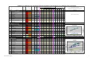
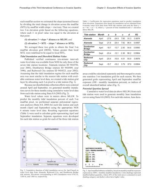
<str<strong>on</strong>g>Proceedings</str<strong>on</strong>g> <str<strong>on</strong>g>of</str<strong>on</strong>g> <str<strong>on</strong>g>the</str<strong>on</strong>g> <str<strong>on</strong>g>Third</str<strong>on</strong>g> <str<strong>on</strong>g>Internati<strong>on</strong>al</str<strong>on</strong>g> <str<strong>on</strong>g>C<strong>on</strong>ference</str<strong>on</strong>g> <strong>on</strong> <strong>Invasive</strong> SpartinaChapter 3: Ecosystem Effects <str<strong>on</strong>g>of</str<strong>on</strong>g> <strong>Invasive</strong> Spartinaeach mudflat secti<strong>on</strong> we estimated <str<strong>on</strong>g>the</str<strong>on</strong>g> slope (assumed linear)by dividing <str<strong>on</strong>g>the</str<strong>on</strong>g> total change in elevati<strong>on</strong> across <str<strong>on</strong>g>the</str<strong>on</strong>g> mudflat(MTL) by mudflat width (slope = rise/run). Then we createdtwo 3-m elevati<strong>on</strong> grids based <strong>on</strong> <str<strong>on</strong>g>the</str<strong>on</strong>g> following equati<strong>on</strong>s,where each 3- m pixel value was equal to <str<strong>on</strong>g>the</str<strong>on</strong>g> elevati<strong>on</strong> atthat point:(1) elevati<strong>on</strong> 1 = slope * distance to MLLW; and(2) elevati<strong>on</strong> 2 = MTL – (slope * distance to MTL).We averaged <str<strong>on</strong>g>the</str<strong>on</strong>g>se two grids to obtain <str<strong>on</strong>g>the</str<strong>on</strong>g> final 3-mmudflat elevati<strong>on</strong> grid (DEM). Values greater than localMTL were redefined to be equal to local MTL.Tidal Inundati<strong>on</strong> and Shorebird Habitat ValuePublished verified c<strong>on</strong>tinuous (six-minute interval)water level data was available from NOS for <strong>on</strong>ly three <str<strong>on</strong>g>of</str<strong>on</strong>g> <str<strong>on</strong>g>the</str<strong>on</strong>g>seven tide stati<strong>on</strong> locati<strong>on</strong>s: Alameda (stati<strong>on</strong> ID 9414750,year 2001), Dumbart<strong>on</strong> Bridge (stati<strong>on</strong> ID 9414509, year1996), and Redwood City (stati<strong>on</strong> ID 9414523, year 2002).Assuming that <str<strong>on</strong>g>the</str<strong>on</strong>g> tidal inundati<strong>on</strong> regime for each mudflatarea was most similar to <str<strong>on</strong>g>the</str<strong>on</strong>g> nearest tide stati<strong>on</strong> with availablec<strong>on</strong>tinous water level data, we created a tide stati<strong>on</strong> gridlayer by allocating each 3-m pixel to a tide stati<strong>on</strong> (Fig. 1).Because our shorebird data collecti<strong>on</strong> efforts were centeredaround April and September, we generated m<strong>on</strong>thly inundati<strong>on</strong>curves for <str<strong>on</strong>g>the</str<strong>on</strong>g>se m<strong>on</strong>ths using cumulative water level datafrom each tide stati<strong>on</strong> using Stata 8.0 (2003) (Fig. 2).Water level values were in meters above MLLW. Topredict <str<strong>on</strong>g>the</str<strong>on</strong>g> m<strong>on</strong>thly tidal inundati<strong>on</strong> percent <str<strong>on</strong>g>of</str<strong>on</strong>g> each 3-mmudflat pixel, we performed separate polynomial regressi<strong>on</strong>analyses (Stata 8.0, 2003) for each tide stati<strong>on</strong> and eachm<strong>on</strong>th (April and September) using <str<strong>on</strong>g>the</str<strong>on</strong>g> appropriate NOS6 minute water level data. Resulting regressi<strong>on</strong> equati<strong>on</strong>s(Table 1) were used to calculate grids representing April andSeptember inundati<strong>on</strong>. Separate equati<strong>on</strong>s were developedfor each tide stati<strong>on</strong> so grids for each <str<strong>on</strong>g>of</str<strong>on</strong>g> <str<strong>on</strong>g>the</str<strong>on</strong>g> three tide stati<strong>on</strong>Table 1. Coefficients for regressi<strong>on</strong> equati<strong>on</strong>s used to predict inundati<strong>on</strong>from elevati<strong>on</strong>. Equati<strong>on</strong>s were based <strong>on</strong> inundati<strong>on</strong> curves obtained from6-minute water level data from NOS tide stati<strong>on</strong>s and took <str<strong>on</strong>g>the</str<strong>on</strong>g> form y =ax + bx 2 + cx 3 + d, where y = percent <str<strong>on</strong>g>of</str<strong>on</strong>g> time inundated and x = elevati<strong>on</strong>above MLLW.Tide stati<strong>on</strong> M<strong>on</strong>th a b c d R2Alameda April -27.9 -24.9 7.85 91.3 0.9974Alameda Sept -21.6 -28.4 7.92 96.4 0.9997Dumbart<strong>on</strong>BridgeApril -19.7 -13.7 2.93 94.6 0.9990Dumbart<strong>on</strong>BridgeSept -20.4 -12.1 2.36 98.2 0.9984RedwoodCityApril -20.4 -16.8 4.01 93.9 0.9974RedwoodCitySept -15.7 -18.2 3.79 97.9 0.9994areas could be calculated separately and <str<strong>on</strong>g>the</str<strong>on</strong>g>n merged to create<strong>on</strong>e seamless 3-m inundati<strong>on</strong> grid for each seas<strong>on</strong>. We <str<strong>on</strong>g>the</str<strong>on</strong>g>ngenerated grids representing April and September mudflatexposure (100 - m<strong>on</strong>thly inundati<strong>on</strong> percent), as indices <str<strong>on</strong>g>of</str<strong>on</strong>g>overall shorebird habitat value (Fig. 3).Potential Spartina SpreadCumulative water level data (m above MLLW) from eachtide stati<strong>on</strong> were used to generate m<strong>on</strong>thly June inundati<strong>on</strong>curves using Stata 8.0 (2003). For each tide stati<strong>on</strong>, June dura-Fig. 2. Cumulative durati<strong>on</strong> <str<strong>on</strong>g>of</str<strong>on</strong>g> tidal inundati<strong>on</strong> curves for April based <strong>on</strong>water level data from Alameda, Redwood City, and Dumbart<strong>on</strong> Bridgetide stati<strong>on</strong>s. Elevati<strong>on</strong>s corresp<strong>on</strong>ding to 60% inundati<strong>on</strong> were 0.762 m,1.018 m, and 1.083 m, respectively.Fig. 3. April mudflat habitat availability, based <strong>on</strong> m<strong>on</strong>thly mudflat exposureexpressed as 100% - m<strong>on</strong>thly mudflat inundati<strong>on</strong>. Color shadings representmudflat habitat quantiles, where 20% <str<strong>on</strong>g>of</str<strong>on</strong>g> <str<strong>on</strong>g>the</str<strong>on</strong>g> total area is c<strong>on</strong>tained in eachshading category and darker colors have higher value.- 177 -