Applied numerical modeling of saturated / unsaturated flow and ...

More documents

Recommendations

Info

(1995) yields a “hybrid” rate constant between a bulk attenuation and a pure biodegradation rate constant, as it accounts for longitudinal dispersion whereas the effects of transverse dispersion are still reflected in the rate constant. A pure biodegradation rate constant can be estimated analytically by normalizing contaminant concentrations to concentrations of a recalcitrant tracer, if such a compound is emitted from the same source zone as the contaminant of concern (Wiedemeier et al. 1996). If this is not the case, an approach of Zhang and Heathcote (2003) may be used, in which the Buscheck and Alcantar (1995) method is extended to account for dispersion in two or three dimensions. Pure biodegradation rate constants exclusive of dispersion or other attenuation processes (and only those) may be used in contaminant transport models for prognoses of plume trends. It is important to note that these center line based rate constant estimation approaches are only applicable to contaminant plumes that have reached steady state conditions, as for still expanding plumes the rate constant would be overestimated. Although it is known, that biodegradation rate estimates obtained from an investigation of the plume center line are subject to substantial uncertainty, this strategy is frequently used in practice. Even in homogeneous aquifers vertical and horizontal transverse dispersion can produce center line concentration profiles of recalcitrant compounds that could be mistaken as following from first order degradation (McNab Jr. and Dooher 1998). Moreover, the plume axis may easily be missed by monitoring wells when the inferred ground water flow direction is incorrect, changes over time due to transient flow behavior or when the contaminant plume shows large scale meandering due to aquifer heterogeneity (Newell et al. 2002; Wilson et al. 2004). Therefore, biodegradation rate constants obtained from such field data should be taken as rough estimates only (Chapelle et al. 2003). As first order rates calculated from center line data include all effects and processes that lower local contaminant concentrations, the precarious result of the different sources of uncertainty is that the degradation potential may be severely overestimated (Rittmann 2004), causing underestimation of plume length and contaminant mass as well as a too optimistic prognosis of down gradient concentrations and exposure levels. These aspects were recently studied in-depth by Bauer et al. (2006a) and Beyer et al. (2006) by means of numerical experiments in two-dimensional synthetic heterogeneous contaminated aquifers. The numerical experiments were based on coarse monitoring networks with 6 to 8 wells, which were all placed along an inferred plume center line. In reality, however, monitoring networks typically are designed to suit multiple and sometimes conflicting requirements and objectives, which may also change with time, depending on the stage of the site investigation. Objectives in this context are the detection of ground water contamination (e.g. Storck et al. 1997), site characterization and spatial delineation of the contamination (e.g. McGrath and Pinder 2003) or the long term monitoring of the plume behavior (e.g. Wu et al. 2006). These aims require spatially more extensive monitoring networks with larger numbers of wells compared to the relatively simple center line well configurations necessary to estimate a degradation rate constant. Recently, Stenback et al. (2004) demonstrated that additional off center line measurements can be incorporated in the estimation of the degradation rate, when a two-dimensional analytical transport model is fitted to contaminant concentrations of all monitoring wells of an extensive monitoring network downgradient from the source. In a field application example Stenback et al. (2004) showed, that accounting for the additional information on contaminant concentrations and distribution significantly reduced rate constant estimates obtained from the conventional center line approach to about 50 %, pointing out the well known problem of rate constant overestimation with the 1D center line method. This paper therefore studies the performance of several rate constant estimation approaches based on center line investigation data for sites with extensive monitoring networks and compares the results to the two-dimensional approach of Stenback et al. (2004). Adopting the terminology of Newell et al. (2002) the types of degradation rate constants regarded here comprise bulk attenuation, biodegradation and “hybrid” rate constants. Point decay rates are not addressed in this paper. Both strategies for rate constant estimation, i.e. the investigation of the plume center line and the approach of Stenback et al. (2004), are applied to a set of synthetic sites with extensive monitoring networks, which were independently designed and installed by individual test persons engaged in hydrogeological research and consulting. The networks were installed for a general characterization and quantification of the contaminant plume (Chen et al. 2005; Bauer et al. 2006b), and are used here as a basis for degradation rate estimation. Estimated rate constants for both strategies are compared with regard to magnitude of errors and variability to draw conclusions on their limitations in view of the monitoring network used. Thereby the studies of Bauer et al. (2006a) and Beyer et al. (2006) are considerably extended, as the monitoring networks used in this paper are representative of real field situations by using all installed observation wells, and are not restricted to an one-dimensional plume center line. Moreover, this analysis allows an evaluation of the “human factor” on estimated rate constants resulting from individual notions of “sufficient accuracy” in plume investigation. Background and Scope This study is based on a set of synthetic contaminated two-dimensional aquifers, generated by multiple stochastic simulations of heterogeneous hydraulic conductivity fields and subsequent numerical simulation of contaminant spreading from a defined source zone in the synthetic aquifers. The evolved virtual plumes were independently investigated by a number of German scientists engaged in hydrogeological and environmental research using an 2
interactive plume investigation and mapping software (Chen et al. 2005) with any number of wells considered necessary for a characterization of the synthetic sites and the delineation of the contaminant plume. The plume investigations were performed within a related project (Bauer et al. 2006b) and are described in detail below. The results of these virtual plume investigations yield individually and realistically investigated plumes. The “measured” concentrations, hydraulic heads and conductivities at the observation well networks of the different plumes investigated are used as a basis for the determination of the degradation rate constants. Two different strategies are compared here: • Strategy A - One-dimensional center line approach: From all observation wells installed the concentration distribution is analyzed and wells along the approximate center line of the contaminant plume are identified (see Figure 1(a)). Concentrations measured in these wells are evaluated using three different methods for the inference of a degradation rate constant (Newell et al. 2002; Buscheck and Alcantar 1995; Zhang and Heathcote 2003). Thus, here only a subset of concentrations measured in the original monitoring network is used for rate constant estimation. • Strategy B - Two-dimensional evaluation: An approximate solution for the two-dimensional steady state concentration distribution is fitted to concentrations measured in all observation wells of the monitoring network downgradient of the source zone using a residual least squares criterion (Stenback et al. 2004) (Figure 1(b)). Fitting parameters are the first order rate constant and the source concentration. 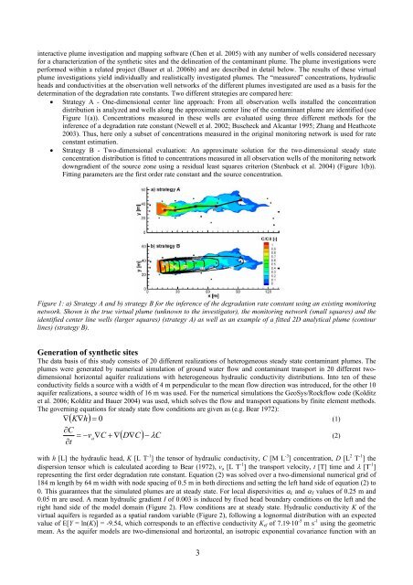Figure 1: a) Strategy A and b) strategy B for the inference of the degradation rate constant using an existing monitoring network. Shown is the true virtual plume (unknown to the investigator), the monitoring network (small squares) and the identified center line wells (larger squares) (strategy A) as well as an example of a fitted 2D analytical plume (contour lines) (strategy B). Generation of synthetic sites The data basis of this study consists of 20 different realizations of heterogeneous steady state contaminant plumes. The plumes were generated by numerical simulation of ground water flow and contaminant transport in 20 different twodimensional horizontal aquifer realizations with heterogeneous hydraulic conductivity distributions. Into ten of these conductivity fields a source with a width of 4 m perpendicular to the mean flow direction was introduced, for the other 10 aquifer realizations, a source width of 16 m was used. For the numerical simulations the GeoSys/Rockflow code (Kolditz et al. 2006; Kolditz and Bauer 2004) was used, which solves the flow and transport equations by finite element methods. The governing equations for steady state flow conditions are given as (e.g. Bear 1972): ∇( K ∇h) = 0 (1) ∂C = −va∇C + ∇( D∇C) − λC (2) ∂t with h [L] the hydraulic head, K [L T -1 ] the tensor of hydraulic conductivity, C [M L -3 ] concentration, D [L 2 T -1 ] the dispersion tensor which is calculated acording to Bear (1972), va [L T -1 ] the transport velocity, t [T] time and λ [T -1 ] representing the first order degradation rate constant. Equation (2) was solved over a two-dimensional numerical grid of 184 m length by 64 m width with node spacing of 0.5 m in both directions and setting the left hand side of equation (2) to 0. This guarantees that the simulated plumes are at steady state. For local dispersivities αL and αT values of 0.25 m and 0.05 m are used. A mean hydraulic gradient I of 0.003 is induced by fixed head boundary conditions on the left and the right hand side of the model domain (Figure 2). Flow conditions are at steady state. Hydraulic conductivity K of the virtual aquifers is regarded as a spatial random variable (Figure 2), following a lognormal distribution with an expected value of E[Y = ln(K)] = -9.54, which corresponds to an effective conductivity Kef of 7.19·10 -5 m s -1 using the geometric mean. As the aquifer models are two-dimensional and horizontal, an isotropic exponential covariance function with an 3
Page 3 and 4:
Applied numerical modeling of satur
Page 5:
Abstract Applied numerical modeling
Page 9:
Vorwort Die zurückliegenden drei J
Page 13:
List of abbreviations and mathemati
Page 16 and 17:
for the application studies outline
Page 18 and 19:
path lengths of water molecules tha
Page 20 and 21:
where vmax [s -1 ] is a maximum gro
Page 22 and 23:
domain is discretized along advecti
Page 24 and 25:
conceptional model error: wrong pro
Page 26 and 27:
The conceptual model used is a rigo
Page 28 and 29:
equires therefore a higher degradat
Page 30 and 31:
studied for heterogeneous sites wit
Page 32 and 33:
Fig. 13: Plume length overestimatio
Page 34 and 35:
concentration maximum is for the ca
Page 36 and 37:
possibilities can not be provided n
Page 38 and 39:
technischen Bauwerken. (Model based
Page 40 and 41:
Schäfer, D., Dahmke, A., Kolditz,
Page 43:
Enclosed Publication 1 Bauer, S., B
Page 46 and 47:
Assessing measurements of first-ord
Page 48 and 49:
Page 50 and 51:
Page 52 and 53:
Page 55 and 56:
WATER RESOURCES RESEARCH, VOL. 42,
Page 57 and 58:
W01420 BAUER ET AL.: ASSESSING FIRS
Page 59 and 60:
Page 61 and 62:
Page 63 and 64: W01420 BAUER ET AL.: ASSESSING FIRS
Page 69: Enclosed Publication 3 Beyer, C., B
Page 72 and 73: 74 C. Beyer et al. / Journal of Con
Page 95: Enclosed Publication 4 Bauer, S., B
Page 98 and 99: Einführung In dieser Arbeit wird e
Page 100 and 101: Entlang der so bestimmten Grundwass
Page 102 and 103: Für die letztgenannten Methoden m
Page 104 and 105: Um diesen Effekt zu verdeutlichen s
Page 106 and 107: Unsicherheit zu. Für Methode 3 ( A
Page 108 and 109: sagt sowie die zusätzliche Problem
Page 111: Enclosed Publication 5 Beyer, C., C
Page 116 and 117: 2 integral scale lY of 2.67 m and l
Page 118 and 119: The approximate solution employed h
Page 120 and 121: As Bauer et al. (2006a) demonstrate
Page 122 and 123: Table 4: Normalized degradation rat
Page 124 and 125: Comparing results for source widths
Page 127: Enclosed Publication 6 Beyer, C., K
Page 130 and 131: Einleitung und Zielsetzung In Deuts
Page 132 and 133: die Anzahl Simulationsläufe den Vo
Page 134 and 135: Grundlage des Korngrößenspektrums
Page 136 and 137: Dies ist als konservative Abschätz
Page 138 and 139: Randbedingungen abhängig ist. Aus
Page 140 and 141: keinen Einfluss auf die abgebaute M
Page 142 and 143: Carsell, R. F., Parish, R. S.: Deve
Page 144: van Genuchten, M.T.: A closed form
show all

Applied numerical modeling of saturated / unsaturated flow and ...

You also want an ePaper? Increase the reach of your titles

Delete template?

Save as template?