Applied numerical modeling of saturated / unsaturated flow and ...

C. Beyer et al. / Journal of Contaminant Hydrology 87 (2006) 73–95
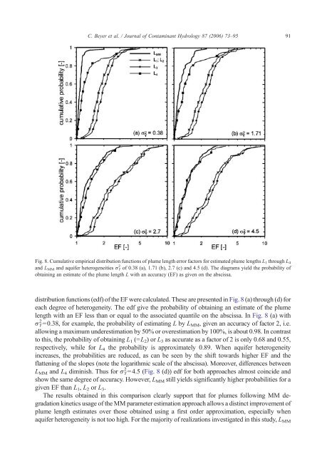
Fig. 8. Cumulative empirical distribution functions of plume length error factors for estimated plume lengths L1 through L4
and LMM and aquifer heterogeneities σY 2 of 0.38 (a), 1.71 (b), 2.7 (c) and 4.5 (d). The diagrams yield the probability of
obtaining an estimate of the plume length L with an accuracy (EF) as given on the abscissa.
distribution functions (edf) of the EF were calculated. These are presented in Fig. 8 (a) through (d) for
each degree of heterogeneity. The edf give the probability of obtaining an estimate of the plume
length with an EF less than or equal to the associated quantile on the abscissa. In Fig. 8 (a) with
σY 2 =0.38, for example, the probability of estimating L by LMM, given an accuracy of factor 2, i.e.
allowing a maximum underestimation by 50% or overestimation by 100%, is about 0.98. In contrast
to this, the probability of obtaining L1 (=L2)orL3 as accurate as a factor of 2 is only 0.68 and 0.55,
respectively, while for L4 the probability is approximately 0.89. When aquifer heterogeneity
increases, the probabilities are reduced, as can be seen by the shift towards higher EF and the
flattening of the slopes (note the logarithmic scale of the abscissa). Moreover, differences between
LMM and L4 diminish. Thus for σY 2 =4.5 (Fig. 8 (d)) edf for both approaches almost coincide and
show the same degree of accuracy. However, LMM still yields significantly higher probabilities for a
given EF than L1, L2 or L3.
The results obtained in this comparison clearly support that for plumes following MM degradation
kinetics usage of the MM parameter estimation approach allows a distinct improvement of
plume length estimates over those obtained using a first order approximation, especially when
aquifer heterogeneity is not too high. For the majority of realizations investigated in this study, L MM
91