

Applied numerical modeling of saturated / unsaturated flow and ...
Applied numerical modeling of saturated / unsaturated flow and ...
Applied numerical modeling of saturated / unsaturated flow and ...

You also want an ePaper? Increase the reach of your titles
YUMPU automatically turns print PDFs into web optimized ePapers that Google loves.
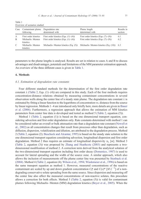
Table 1<br />
Overview <strong>of</strong> scenarios studied<br />
Case Contaminant plume<br />
following<br />
parameters to the plume lengths is analysed. Results are set in relation to cases A <strong>and</strong> B to discuss<br />
advantages <strong>and</strong> disadvantages, potentials <strong>and</strong> limitations <strong>of</strong> the MM parameter estimation approach.<br />
An overview <strong>of</strong> the three different cases is given in Table 1.<br />
4. Methods<br />
C. Beyer et al. / Journal <strong>of</strong> Contaminant Hydrology 87 (2006) 73–95<br />
Degradation rate<br />
determined with<br />
4.1. Estimation <strong>of</strong> degradation rate constants<br />
Plume length<br />
determined with<br />
A First order kinetics First order kinetics (Eqs. (1)–(4)) First order kinetics (Eqs. (7)–(9)) 6.1<br />
B Michaelis–Menten<br />
kinetics<br />
First order kinetics (Eqs. (1)–(4)) First order kinetics (Eqs. (7)–(9)) 6.2<br />
C Michaelis–Menten<br />
kinetics<br />
Michaelis–Menten kinetics (Eq. (5)) Michaelis–Menten kinetics (Eq. (10)) 6.3<br />
Results in<br />
section<br />
Four different st<strong>and</strong>ard methods for the determination <strong>of</strong> the first order degradation rate<br />
constant λ (Table 2, Eqs. (1)–(4)) are compared in this study. Each <strong>of</strong> the four methods requires<br />
concentration-distance relations obtained by measuring contaminant concentrations in several<br />
observation wells along the center line <strong>of</strong> a steady state plume. The degradation rate constant λ is<br />
estimated by fitting a linear function to the logarithms <strong>of</strong> concentration vs. distance from the source<br />
by linear regression. Methods 1–4 are introduced only briefly here, more details are given in Bauer<br />
et al. (2006). Furthermore, a regression approach that allows the estimation <strong>of</strong> MM kinetics<br />
parameters from center line data is developed <strong>and</strong> tested as method 5 (Table 2, equation (5)).<br />
Method 1 (Table 2, equation (1)) is based on the one dimensional transport equation, considering<br />
advection <strong>and</strong> first order degradation only. Rate constants determined with method 1 can<br />
be considered rather an overall or bulk attenuation rate than a degradation rate constant (Newell et<br />
al., 2002) as all concentration changes that result from processes other than degradation, such as<br />
diffusion, dispersion, volatilization <strong>and</strong> dilution, are attributed to the degradation process. Method<br />
2(Table 2, equation (2); Buscheck <strong>and</strong> Alcantar, 1995) is based on the steady state solution to the<br />
one dimensional transport equation considering advection, longitudinal dispersion <strong>and</strong> first order<br />
degradation. Method 2 thus requires an estimate <strong>of</strong> longitudinal dispersivity αL [m]. Method 3<br />
(Table 2, equation (3)) was proposed by Zhang <strong>and</strong> Heathcote (2003) <strong>and</strong> represents a twodimensional<br />
modification <strong>of</strong> method 2. A correction term derived from the analytical solution <strong>of</strong><br />
the two-dimensional transport equation including first order decay (Domenico, 1987) is used to<br />
account for lateral spreading <strong>and</strong> the width <strong>of</strong> the source zone. A similar approach, which also<br />
allows the inclusion <strong>of</strong> measurements <strong>of</strong>f the plume center line was presented by Stenback et al.<br />
(2004). Method 4 (Table 2, equation (4); Wilson et al., 1994; Wiedemeier et al., 1996) is based on<br />
the same transport equation as method 1. However, measured concentrations <strong>of</strong> the reactive<br />
contaminant are scaled by up <strong>and</strong> down gradient concentration C0 ⁎ <strong>and</strong> C(x)⁎ [M L − 3 ] <strong>of</strong> a nondegrading<br />
conservative solute spreading from the same source. Since dispersion <strong>and</strong> measuring <strong>of</strong>f<br />
the center line also affect the measured concentrations <strong>of</strong> non-reactive solutes, this procedure<br />
allows a correction for both effects. Method 5 (Table 2, equation (5)) is valid for contaminant<br />
plumes following Michaelis–Menten (MM) degradation kinetics (Beyer et al., 2005). When the<br />
77


