Applied numerical modeling of saturated / unsaturated flow and ...

W01420 BAUER ET AL.: ASSESSING FIRST-ORDER RATES
the first-order degradation rate constants by the four methods
presented above. The investigation setup is designed to
resemble ideal conditions for the application of the four
methods for estimating the degradation rate constant. All
measurements are assumed to be exact, which means that
there is no measurement error involved. The only uncertainty
and variability is introduced by the heterogeneity of
hydraulic conductivity. For methods 3 and 4, additionally
aL and aT have to be known. These are estimated following
Wiedemeier et al. [1999] as 0.1 of the plume length for aL,
with aT being about 0.33 of the longitudinal dispersivity. As
plume length the maximum distance covered by the observation
wells, i.e., 30 m, is used. As the plumes are generally
longer, this assumption yields rather low dispersivities.
Thus aL and aT are estimated to be 3.0 and 1.0 m,
respectively. These estimates of dispersivities are not optimal,
as they are not based on the heterogeneity of the
hydraulic conductivity. However, dispersivities based on
results from stochastic hydrogeology are difficult to obtain,
as for most field sites structure and degree of heterogeneity
are not well known. Also, the four samples taken in this
investigation scenario do not allow for an estimation of the
correlation length or the ln(K) variances. Both the correct
source width and the correct porosity are used. In the last
step, by each of the four approaches the corresponding
first-order degradation rate constants l 1 through l 4 are
calculated. These values can be compared to the value used
to generate the plume (l =1a 1 ). For each realization, the
investigation procedure described above is followed and a
degradation rate is calculated for each method, each downstream
well and for each source width. For each of the four
classes of heterogeneity used in this study (ln(K) variances
s Y 2 of 0.38, 1.71, 2.70 and 4.50) a minimum of 100 realizations
is evaluated. Thus statistical measures of the errors
and uncertainties introduced by the heterogeneity of the
hydraulic conductivity are obtained. Additionally, also the
impact of the width of the source zone is studied. Here it
is expected, that for increasing source width the onedimensional
methods yield better results, as then the
investigated situation corresponds better to the assumptions
of the method. Source widths W S of 4 m, 8 m and 16 m are
used, corresponding to 1.5, 3 and 6 integral scales l Y. Then
methods for estimating the flow velocity are elucidated for
the different degrees of heterogeneity. This is because the
goodness of the calculated value for lambda is directly
related to estimated transport velocity accuracy. Finally the
influence of estimated longitudinal and transversal dispersivities
on results by methods 3 and 4 is studied in a
sensitivity analysis.
2.4. Numerical Tests
[16] Convergence of the Monte Carlo simulation with
regard to the sample size N of estimated degradation rate
constants was tested by a procedure following Goovaerts
[1999]. The test is only conducted for the highest degree of
heterogeneity used in this study (sY 2 = 4.5) and the smallest
source width of 4 m, as this is the case of highest variability.
A total of 1000 realizations of the random conductivity field
was generated. For each realization, plume development
was simulated and the degradation rate constant l1 was
calculated using method 1. The resulting set of 1000
degradation rates is assumed to be sufficiently large to
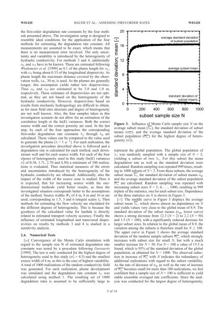
Figure 3. Influence of Monte Carlo sample size N on the
average subset mean (l1), the standard deviation of subset
means (sl1 ), and the average standard deviation of the
subset population (sl1 ) for the highest degree of heterogeneity
(sY 2 ).
represent the global population. The global population of
l1 was randomly sampled with a sample size of N =2,
yielding a subset of two l1. For this subset the mean
degradation rate as well as the standard deviation were
calculated. Random sampling was repeated 999 times, resulting
in 1000 subsets of N = 2. From these subsets, the average
subset mean l1, the standard deviation of subset means sl1 and the average standard deviation of the subset population
sl1 are calculated. Random sampling was repeated with
increasing subset sizes N =3,4,..., 1000, resulting in 999
triplets of the statistics, one for each subset size. Dependence
of the three statistics on N is shown in Figure 3.
[17] The middle curve in Figure 3 displays the average
subset mean l1, which shows almost no dependence on N
and yields values very close to the global mean of 8.9. The
standard deviation of the subset means (s , lower curve)
l1
shows a strong decrease from 12.3 (N = 2) to 2.2 (N = 50)
and 1.5 (N = 100), with a significantly reduced decrease for
larger subset sizes. In relation to the global mean of 8.9, the
variation among the subsets is therefore small for N 100.
The upper curve in Figure 3 shows the average standard
deviation of the random sample subsets sl1 , which strongly
increases with subset size for small N, but with a much
smaller increase for N > 50. For N = 100 a value of 15.5 is
found, which is 95% of the standard deviation of the global
population, as obtained for N = 1000. The observed reduction
in increase of sl1 with N indicates the redundancy of
additional realizations with regard to the subset variability.
As the rate of decrease of s as well as the rate of increase
l1
of sl1 becomes small for more than 100 realizations, we feel
confident that a sample size of N = 100 is sufficient to yield
stable ensemble averaged rate coefficients. Since the analysis
was conducted for the largest degree of heterogeneity,
5of14
W01420