Applied numerical modeling of saturated / unsaturated flow and ...

More documents

Recommendations

Info

84 C. Beyer et al. / Journal of Contaminant Hydrology 87 (2006) 73–95 The overestimation observed for the different Λi results from a combination of several effects. Method 1, which is the simplest approach used in this study, is based on the one dimensional transport equation only accounting for advection and degradation. Concentration reductions on the plume center line caused by transverse dispersion therefore are incorrectly attributed to the degradation process and Λ1 is overestimated. Moreover, when the inferred center line deviates from the true center line, concentrations measured are too low, which further increases rate overestimation. A third source of error is the estimate of v a (see Section 5), which may not be representative for the flow path. Overestimation is caused if v a is estimated too high, while a too low value of v a causes underestimation of the rate constant. All three error types are also relevant for method 2. The additional bias of method 2 towards too large rate constants in comparison with method 1 is a consequence of accounting for αL in equation (2) of Table 2. Longitudinal dispersion of a degrading contaminant results in a stronger spreading of the solute down stream and consequently in higher concentrations along the center line of a steady state plume. Equation (2) can be rearranged to show that λ2=λ1+αLva(ln(C(x)/C0)/Δx) 2 , i.e. λ2 grows linearly with αL and is always larger than λ1 for αLN0.Method3isaffectedbyerrorsinva and off center line measurements. By accounting for transverse dispersion, rate constant estimates are improved compared to method 2, because βb1.0 in equation (4) and thus Λ 3bΛ 2 always. 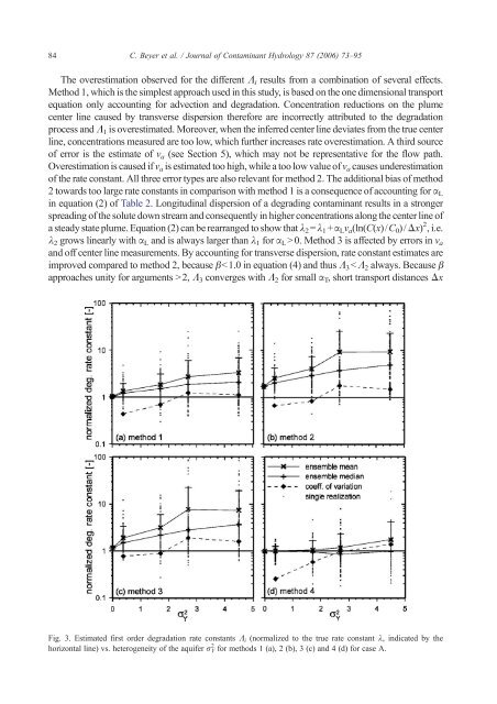Because β approaches unity for arguments N2, Λ3 converges with Λ2 for small αT, short transport distances Δx Fig. 3. Estimated first order degradation rate constants Λi (normalized to the true rate constant λ, indicated by the horizontal line) vs. heterogeneity of the aquifer σ Y 2 for methods 1 (a), 2 (b), 3 (c) and 4 (d) for case A.
C. Beyer et al. / Journal of Contaminant Hydrology 87 (2006) 73–95 and large source widths WS. A surprising result is that method 1, despite its simplicity, yields closer estimates of the true rate constant than the more comprehensive description by method 3. Since method 3 depends on longitudinal and transverse dispersivities, an adequate parameterization is crucial for its success. From stochastic hydrogeology it is known that αL as well as αT strongly depends on travel time and distance as well as on the correlation structure of hydraulic conductivity and flow velocity (e.g. Dagan, 1989). Consequently, a uniform parameterization solely based on the scale of the contaminant problem as used in this study (and with many field applications) is not adequate. A detailed sensitivity study on the influence of dispersivity parameterization on the performance of methods 2 and 3 is presented in Bauer et al. (2006). It is found that for method 2 no value of αL and for method 3 only very high and thus unphysical values of αT yield the correct degradation rate constant. The required values, however, cannot be deduced from aquifer heterogeneity σY 2 alone, as the other errors also influence the estimated degradation rate constant. Method 4 circumvents this problem and corrects for transverse dispersion as well as for measuring off the center line by normalizing concentrations to a conservative tracer. The bias towards too large degradation rate constants observed for the other methods is significantly reduced yielding the closest estimates of λ of the four methods. The remaining deviation from the true rate constant is due to the hydraulic error introduced by the approximation of va. For low heterogeneities there is no evidence for a systematic bias towards either too high or too low rate constants. A prerequisite which may limit the applicability of method 4 is the presence of a suited normalization compound. A discussion of potential normalization compounds is provided in U.S. EPA (1998) and Wiedemeier et al. (1996, 1999). 6.1.2. Estimation of plume lengths During site characterization, estimating degradation rate constants rarely is a goal per se. Here, the kinetics of contaminant degradation are quantified to be used for prediction of the steady state length of the plumes. In site assessment, such information could be used to identify potential receptors and exposure levels. Rate constants λ1, λ2 and λ3 are evaluated using the respective corresponding equations (7), (8) and (9) of Table 3 yielding plume length estimates L1, L2 and L3. Forλ4 also equation (9) is used yielding L4. To be able to compare the results of all realizations, the Li are normalized by the respective true length L read from the model output. Resulting over- respectively underestimation factors against aquifer heterogeneity σY 2 are presented in Fig. 4 (single realization results, ensemble means with standard deviations as error bars, medians, coefficients of variation). Plume lengths L 1 and L 2, calculated from λ 1 and λ 2, show exactly identical results, although the λ2 show a stronger overestimation than the corresponding λ1 for all realizations. The reason for the equivalence of L1 and L2 is that the bias introduced by estimating λ2 with a one dimensional model accounting for longitudinal dispersion only is reversed by using the same transport equation to calculate the plume length. While for homogeneous conditions the true plume length is obtained, L is underestimated in most realizations for all degrees of heterogeneity. Mean L1 and L2 decrease to 0.59 for σY 2 =4.5. As for λ, spread and uncertainty of L increase with σ Y 2 . The overestimation of the degradation rate constant is thus reflected in an underestimation of the plume length. Plume lengths L3 calculated with the two-dimensional transport equation on average are lower than the corresponding L1 and L2. This is a consequence of the β term in equation (5) (Table 2), which is used to correct down gradient concentrations for transverse dispersion. When estimating the rate constant with method 3, each down gradient concentration C(x) is scaled by a different value β, as the correction factor is dependent on the distance from the source. This scaling is not fully reversed when the plume length is calculated using equation (9) (Table 3), as then only one single Δx is used. 85
Page 3 and 4:
Applied numerical modeling of satur
Page 5:
Abstract Applied numerical modeling
Page 9:
Vorwort Die zurückliegenden drei J
Page 13:
List of abbreviations and mathemati
Page 16 and 17:
for the application studies outline
Page 18 and 19:
path lengths of water molecules tha
Page 20 and 21:
where vmax [s -1 ] is a maximum gro
Page 22 and 23:
domain is discretized along advecti
Page 24 and 25:
conceptional model error: wrong pro
Page 26 and 27:
The conceptual model used is a rigo
Page 28 and 29:
equires therefore a higher degradat
Page 30 and 31:
studied for heterogeneous sites wit
Page 32 and 33: Fig. 13: Plume length overestimatio
Page 34 and 35: concentration maximum is for the ca
Page 36 and 37: possibilities can not be provided n
Page 38 and 39: technischen Bauwerken. (Model based
Page 40 and 41: Schäfer, D., Dahmke, A., Kolditz,
Page 43: Enclosed Publication 1 Bauer, S., B
Page 46 and 47: Assessing measurements of first-ord
Page 55 and 56: WATER RESOURCES RESEARCH, VOL. 42,
Page 57 and 58: W01420 BAUER ET AL.: ASSESSING FIRS
Page 69: Enclosed Publication 3 Beyer, C., B
Page 72 and 73: 74 C. Beyer et al. / Journal of Con
Page 95: Enclosed Publication 4 Bauer, S., B
Page 98 and 99: Einführung In dieser Arbeit wird e
Page 100 and 101: Entlang der so bestimmten Grundwass
Page 102 and 103: Für die letztgenannten Methoden m
Page 104 and 105: Um diesen Effekt zu verdeutlichen s
Page 106 and 107: Unsicherheit zu. Für Methode 3 ( A
Page 108 and 109: sagt sowie die zusätzliche Problem
Page 111: Enclosed Publication 5 Beyer, C., C
Page 114 and 115: (1995) yields a “hybrid” rate c
Page 116 and 117: 2 integral scale lY of 2.67 m and l
Page 118 and 119: The approximate solution employed h
Page 120 and 121: As Bauer et al. (2006a) demonstrate
Page 122 and 123: Table 4: Normalized degradation rat
Page 124 and 125: Comparing results for source widths
Page 127: Enclosed Publication 6 Beyer, C., K
Page 130 and 131: Einleitung und Zielsetzung In Deuts
Page 132 and 133:
die Anzahl Simulationsläufe den Vo
Page 134 and 135:
Grundlage des Korngrößenspektrums
Page 136 and 137:
Dies ist als konservative Abschätz
Page 138 and 139:
Randbedingungen abhängig ist. Aus
Page 140 and 141:
keinen Einfluss auf die abgebaute M
Page 142 and 143:
Carsell, R. F., Parish, R. S.: Deve
Page 144:
van Genuchten, M.T.: A closed form
show all

Applied numerical modeling of saturated / unsaturated flow and ...

Create successful ePaper yourself

Delete template?

Save as template?