Applied numerical modeling of saturated / unsaturated flow and ...

Steps 1 and 2 could be repeated as often as desired by the investigator, until the interpolated contaminant plume was
deemed to be investigated accurately enough to properly characterize the contaminant distribution. Thus the interactive
site investigation is an iterative procedure and is evaluated by a comparison of the “true” plume with the investigation
result. More details on this procedure can be found in Chen et al. (2005).
Using this methodology, a total number of 85 individual investigation results were obtained. 47 of these investigations
were conducted for plumes originating from a source of width 4 m, while the plumes with a source width of 16 m were
investigated 38 times. Accordingly, the majority of the 20 different plumes were investigated three or four times by
different investigators.
The configuration and the number of monitoring wells varies substantially between the different realizations and even for
the same realization but different investigators (12 – 93 wells), as the decision about how many wells were needed for an
accurate characterization of the site was left to the individual investigators. For two contaminant plumes (one for each
source width) the investigation was repeated 13 times. Each investigation was performed by a different investigator. In
addition to the general comparison of strategies A and B for the inference of the degradation rate constant, this subset of
the whole data set allows for an analysis of estimated rate constant variability for a single site, resulting from different
notions of “sufficient accuracy” of the virtual plume investigation.
Rate constant estimation
Using the monitoring networks installed by the investigators of the virtual plumes, first order rate constants were
estimated following strategies A and B. Methods A1, A2 and A3 are used in strategy A and are described in detail in
Bauer et al. (2006a). Therefore, only a brief description is given here:
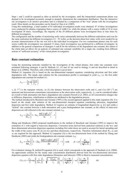
Method A1 (equation (3)) is based on the one-dimensional transport equation, considering advection and first order
degradation only. The steady state solution for the concentration profile is rearranged to yield λA1, i.e. the first order
degradation rate constant for method A1:
va ⎛ C(
x)
⎞
λ A1
= − ln⎜ ⎟
∆x
⎜ ⎟
(3)
⎝ C0
⎠
va [L T -1 ] is the transport velocity, ∆x [L] the distance between the observation wells and C0 and C(x) [M L -3 ] are
upstream and downstream contaminant concentrations at the observation wells, respectively. λA1 can be considered rather
an overall or bulk attenuation rate than a degradation rate constant (Newell et al. 2002), as all concentration changes due
to diffusion, dispersion, volatilization or dilution are attributed to the degradation process.
The method introduced by Buscheck and Alcantar (1995) is the second approach applied in this study (equation (4)). It is
based on the steady state solution of the one-dimensional transport equation considering advection, longitudinal
dispersion and first order degradation. Method A2 requires an estimate of longitudinal dispersivity αL [L] and yields a
“hybrid” rate constant between a bulk attenuation and a pure biodegradation rate constant, as the effects of transverse
dispersion are still reflected in the rate constant estimate λA2.
⎛
2
v
( ) ⎞
a ⎜⎛
ln C(
x)
C0
⎞
λ = ⎜1
− 2
⎟ −1⎟
A2
α L
4α
⎜
⎟
L ⎝⎝
∆x
⎠ ⎠
(4)
Zhang and Heathcote (2003) proposed modifications to the method of Buscheck and Alcantar (1995) to improve the
estimation of λ with regard to transverse dispersion. Correction terms derived from analytical solutions to the two- and
three-dimensional advection dispersion equations including first order decay are used to account for lateral spreading and
the width of the source zone WS [L] in two and three dimensions, respectively. Therefore information about WS, αL and
αT are required for this approach. Method A3 (equation (5)) is the two-dimensional form of the method by Zhang and
Heathcote (2003) and yields the biodegradation rate constant estimate λA3:
2
v ⎛ ( ) ⎞
a ⎜⎛
ln C(
x)
( C0β
) ⎞
⎛ ⎞
λ = − ⎟
A3
⎜
⎜1−
2α
L
⎟ 1 with
⎜ WS
β = erf ⎟ (5)
4α
⎟
L ⎝⎝
∆x
⎠
⎜ ⎟
⎠
⎝ 4 αT
∆x
⎠
For evaluation strategy B, method B (equation (6)) is used, which corresponds to the approach of Stenback et al. (2004).
An approximate solution for the steady state concentration distribution derived from the two-dimensional advectiondispersion
equation with first order degradation (Domenico and Schwartz 1990) is fitted to measured concentrations:
C ⎪⎧
⎛
⎞⎪⎫
⎪
⎧ ⎛ ⎞ ⎛ ⎞⎪
⎫
0 ⎛ x ⎞
⎨
⎜ + ⎟ ⎜ −
⎨ ⎜
4λ
⎟⎬
−
⎟
⎜
⎟
Bα
L 2y
WS
2y
WS
C(
x,
y)
= exp 1−
1+
erf
erf ⎬ (6)
2 ⎪⎩ ⎝ 2α
⎠
⎜
⎟
⎪⎭ ⎪⎩
⎜ ⎟ ⎜ ⎟
L ⎝
va
⎠ ⎝ 4 αT
x ⎠ ⎝ 4 αT
x ⎠⎪⎭
5