Applied numerical modeling of saturated / unsaturated flow and ...

W01420 BAUER ET AL.: ASSESSING FIRST-ORDER RATES
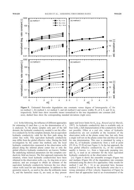
Figure 5. Estimated first-order degradation rate constants versus degree of heterogeneity sY 2 for
(a) method 1, (b) method 2, (c) method 3, and (d) method 4 and source widths WS of 4, 8, and 16 m,
respectively. Solid lines show ensemble means normalized to the true degradation rate constant (left
axis), dashed lines show the corresponding standard deviations (right axis).
[29] In the following, the influence of different approaches
for estimating K (and thus va) on the determination of li
is analyzed. As the plume samples only part of the full
domain, the hydraulic conductivity needed is not the effective
conductivity for the complete domain, but an equivalent
hydraulic conductivity valid for the flow path along the
center line wells. This equivalent hydraulic conductivity
may differ from the global effective value. During the field
investigation by the center line method, only the local
hydraulic conductivities measured at the observation wells
placed along the inferred plume center line or only the
global effective hydraulic conductivity are known. Neither
the underlying statistical parameters nor the complete conductivity
field are known. The first approach represents the
situation, where local hydraulic conductivities have been
obtained in the observation wells, e.g., by slug tests or sieve
analysis, and are averaged to obtain an estimate of the
equivalent hydraulic conductivity between the two observation
wells used for rate determination. In addition to the
geometric mean Kg, as used so far, also the arithmetic mean
Ka and the harmonic mean Kh are used, as they present
9of14
W01420
upper and lower limits for Kef [e.g., Renard and de Marsily,
1997]. As hydraulic conductivity data is available only at
four wells, a full characterization of the conductivity field is
not possible. Often at a real site, values of hydraulic
conductivity are not available at the locations of the
observation wells at the plume center line, but only from
a single well not on the plume center line and thus not used
for rate determination. This case is simulated by using a
value KS of hydraulic conductivity from a well at point
[55.10 m, 55.20 m] (see Figure 1). In the last approach, the
true global effective conductivity KG of the synthetic
aquifer is known, i.e., from a large-scale pumping test,
and KG is used as an estimator for the local equivalent
hydraulic conductivity at the observation wells.
[30] Figure 6 shows the ensemble averages (Figure 6a)
and medians (Figure 6b) of the degradation rate constants
estimated using the above five approaches. Only results for
method 2 and WS = 16 m are presented here, because
method 2 is only affected by the hydraulic error due to a
wrong estimation of flow velocity. Inspection of Figure 6a
shows that all approaches lead to an overestimation of the